3.3 Consistent estimators

The concept of consistency is related with the sample size \(n.\) Assume that \(X\) is a rv with induced probability \(\mathbb{P}(\cdot;\theta),\) \(\theta\in\Theta,\) and that \((X_1,\ldots,X_n)\) is a srs of \(X.\) Take an estimator \(\hat{\theta}\equiv\hat{\theta}(X_1,\ldots,X_n),\) where we have emphasized the dependence of the estimator on the srs. Of course \(\hat{\theta}\) depends on \(n\) and, to remark that, we will also denote the estimator by \(\hat{\theta}_n.\) The question now is: what happens with the distribution of this estimator as the sample size increases? Is its distribution going to be more concentrated around the true value \(\theta\)?

We will study different concepts of consistency, all of them taking into account the distribution of \(\hat{\theta}.\) The first concept we will see tell us that an estimator is consistent in probability if the probability of \(\hat{\theta}\) being far away from \(\theta\) decays as \(n\to\infty.\)

Example 3.11 Let \(X\sim \mathcal{N}(\mu,\sigma^2).\) Let us see how the distribution of \(\bar{X}-\mu\) changes as \(n\) increases, for \(\sigma=2.\)

We know from Theorem 2.1 that

\[\begin{align*} Z=\frac{\bar{X}-\mu}{\sigma/\sqrt{n}}\sim\mathcal{N}(0,1). \end{align*}\]

From that result, we have computed below the probabilities \(\mathbb{P}\left(\vert\bar{X}_n-\mu\vert>\varepsilon\right)=2\mathbb{P}\left(Z>\frac{\varepsilon}{\sigma/\sqrt{n}}\right)\) for \(\varepsilon_1=1\) and \(\varepsilon_2=0.5.\)

\(n\)	\(\bar{X}_n\)	\(\mathbb{P}\left(\vert\bar{X}_n-\mu\vert>1\right)\)	\(\mathbb{P}\left(\vert\bar{X}_n-\mu\vert>0.5\right)\)
\(1\)	\(X_1\)	\(0.6171\)	\(0.8026\)
\(2\)	\(\sum_{i=1}^2X_i/2\)	\(0.4795\)	\(0.7237\)
\(3\)	\(\sum_{i=1}^3X_i/3\)	\(0.3865\)	\(0.6650\)
\(10\)	\(\sum_{i=1}^{10} X_i/10\)	\(0.1138\)	\(0.4292\)
\(20\)	\(\sum_{i=1}^{20} X_i/20\)	\(0.0253\)	\(0.2636\)
\(50\)	\(\sum_{i=1}^{50} X_i/50\)	\(0.0004\)	\(0.0771\)

Observe that \(\bar{X}_n\) is a sequence of estimators of \(\mu\) indexed by \(n.\) Moreover, the probabilities shown in the table also form a sequence. This sequence of probabilities decreases to zero as we increase the sample size \(n.\) This convergence towards zero happens irrespective of the value of \(\varepsilon,\) despite the sequence of probabilities for \(\varepsilon_2\) being larger than the one for \(\varepsilon_1,\) for each \(n,\) since \(\varepsilon_2\leq \varepsilon_1.\) Figure 3.3 shows the evolution of the “\(\bar{X}_n\) is \(\varepsilon\) units far away from \(\mu\)” probabilities for several \(\varepsilon\)’s.

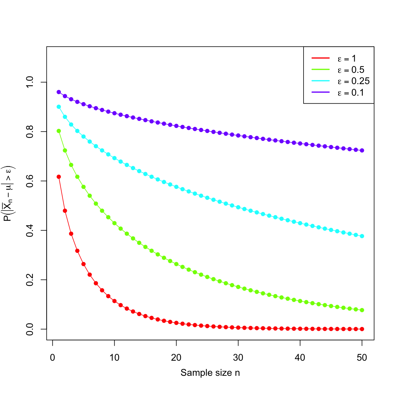
Figure 3.3: Probability sequences \(n\mapsto\mathbb{P}\left(\vert\bar{X}_n-\mu\vert>\varepsilon\right)\) for a \(\mathcal{N}(\mu,\sigma^2)\) with \(\sigma=2\).

Then, an estimator \(\hat{\theta}\) for \(\theta\) is consistent in probability when the probabilities of \(\hat{\theta}\) and \(\theta\) differing more than \(\varepsilon>0\) decrease as \(n\to\infty.\) Or, equivalently, when the probabilities of \(\hat{\theta}\) and \(\theta\) being closer than \(\varepsilon\) grow as \(n\) increases. This must happen for any \(\varepsilon>0.\) If this is true, then the distribution of \(\hat{\theta}\) becomes more and more concentrated about \(\theta.\)

Definition 3.5 (Consistency in probability) Let \(X\) be a rv with induced probability \(\mathbb{P}(\cdot;\theta).\) Let \((X_1,\ldots,X_n)\) be a srs of \(X\) and let \(\hat{\theta}_n\equiv\hat{\theta}_n(X_1,\ldots,X_n)\) be an estimator of \(\theta.\) The sequence \(\{\hat{\theta}_n:n\in\mathbb{N}\}\) is said to be consistent in probability (or consistent) for \(\theta,\) if

\[\begin{align*} \forall \varepsilon>0, \quad \lim_{n\to\infty} \mathbb{P}\big(|\hat{\theta}_n-\theta|>\varepsilon\big)=0. \end{align*}\]

We simply say that the estimator \(\hat{\theta}_n\) is consistent in probability to indicate that the sequence \(\{\hat{\theta}_n:n\in\mathbb{N}\}\) is consistent in probability.

Example 3.12 Let \(X\sim\mathcal{U}(0,\theta)\) and let \((X_1,\ldots,X_n)\) be a srs of \(X.\) Show that the estimator \(\hat{\theta}_n=X_{(n)}\) is consistent in probability for \(\theta.\)

We take \(\varepsilon>0\) and compute the limit of the probability given in Definition 3.5. Since \(\theta \geq X_i,\) \(i=1,\ldots,n,\) we have that

\[\begin{align*} \mathbb{P}\big(|\hat{\theta}_n-\theta|>\varepsilon\big)=\mathbb{P}(\theta-X_{(n)}>\varepsilon)=\mathbb{P}\left(X_{(n)}<\theta-\varepsilon\right)=F_{X_{(n)}}(\theta-\varepsilon). \end{align*}\]

If \(\varepsilon>\theta,\) then \(\theta-\varepsilon<0\) and therefore \(F_{X_{(n)}}(\theta-\varepsilon)=0.\) For \(\varepsilon\leq\theta,\) the cdf evaluated at \(\theta-\varepsilon\) is not zero. Using Example 3.3:

\[\begin{align*} F_{X_{(n)}}(x)=\left(F_X(x)\right)^n=\left(\frac{x}{\theta}\right)^n, \quad x\in(0,\theta). \end{align*}\]

Considering the value of such distribution at \(\theta-\varepsilon\in [0,\theta),\) we get

\[\begin{align*} F_{X_{(n)}}(\theta-\varepsilon)=\left(\frac{\theta-\varepsilon}{\theta}\right)^n=\left(1-\frac{\varepsilon}{\theta}\right)^n. \end{align*}\]

Then, taking the limit as \(n\to\infty\) and noting that \(\varepsilon<\theta,\) we have

\[\begin{align*} \lim_{n\to\infty} \mathbb{P}\big(|\hat{\theta}_n-\theta|>\varepsilon\big)=\lim_{n\to\infty}\left(1-\frac{\varepsilon}{\theta}\right)^n=0. \end{align*}\]

We have shown that \(\hat{\theta}_n=X_{(n)}\) is consistent in probability for \(\theta.\)

The concept of consistency in probability of a sequence of estimators can be extended to general sequences of rv’s. This gives an important type of convergence of rv’s, the convergence in probability.³³

Definition 3.6 (Convergence in probability) A sequence \(\{X_n:n\in\mathbb{N}\}\) of rv’s defined over the same measurable space \((\Omega,\mathcal{A},\mathbb{P})\) is said to converge in probability to another rv \(X,\) and is denoted by

\[\begin{align*} X_n \stackrel{\mathbb{P}}{\longrightarrow} X, \end{align*}\]

if the following statement holds:

\[\begin{align*} \forall \varepsilon>0, \quad \lim_{n\to\infty} \mathbb{P}(|X_n-X|>\varepsilon)=0, \end{align*}\]

where here \(\mathbb{P}\) stands for the joint induced probability function of \(X_n\) and \(X.\)

The following definition establishes another type of consistency that is stronger than (in the sense that implies, but it is not implied) consistency in probability.

Definition 3.7 (Consistency in squared mean) A sequence of estimators \(\{\hat{\theta}_n:n\in\mathbb{N}\}\) is consistent in squared mean for \(\theta\) if

\[\begin{align*} \lim_{n\to\infty}\mathrm{MSE}\big[\hat{\theta}_n\big]=0, \end{align*}\]

or, equivalently, if

\[\begin{align*} \lim_{n\to\infty} \mathrm{Bias}\big[\hat{\theta}_n\big]=0 \quad \text{and}\quad \lim_{n\to\infty} \mathbb{V}\mathrm{ar}\big[\hat{\theta}_n\big]=0. \end{align*}\]

Example 3.13 In a \(\mathcal{U}(0,\theta)\) population, let us check if \(\hat{\theta}_n=X_{(n)}\) is consistent in squared mean for \(\theta.\)

The MSE of \(\hat{\theta}_n\) is given by³⁴

\[\begin{align*} \mathrm{MSE}\big[\hat{\theta}_n\big]=\mathbb{E}\big[(\hat{\theta}_n-\theta)^2\big]=\mathbb{E}\big[\hat{\theta}_n^2-2\theta\hat{\theta}_n+\theta^2\big]. \end{align*}\]

Therefore, we have to compute the expectation and variance of \(\hat{\theta}_n=X_{(n)}.\) Example 3.3 gave the density and expectation of \(\hat{\theta}_n=X_{(n)}\):

\[\begin{align*} f_{\hat{\theta}_n}(x)=\frac{n}{\theta}\left(\frac{x}{\theta}\right)^{n-1}, \quad x\in(0,\theta), \quad \mathbb{E}\big[\hat{\theta}_n\big]=\frac{n}{n+1}\theta. \end{align*}\]

It remains to compute

\[\begin{align*} \mathbb{E}\big[\hat{\theta}_n^2\big]&=\int_0^{\theta} x^2 \frac{n}{\theta}\left(\frac{x}{\theta}\right)^{n-1}\,\mathrm{d}x\\ &=\frac{n}{\theta^n} \int_0^{\theta} x^{n+1}\,\mathrm{d}x=\frac{n}{\theta^n}\frac{\theta^{n+2}}{n+2}= \frac{n\theta^2}{n+2}. \end{align*}\]

Then, the MSE is

\[\begin{align*} \mathrm{MSE}\big[\hat{\theta}_n\big]=\left(1-\frac{2n}{n+1}+\frac{n}{n+2}\right)\theta^2. \end{align*}\]

Taking the limit as \(n\to\infty,\) we obtain

\[\begin{align*} \lim_{n\to\infty} \mathrm{MSE}\big[\hat{\theta}_n\big]=0, \end{align*}\]

so \(\hat{\theta}_n=X_{(n)}\) is consistent in squared mean (even if it is biased).

From the previous definition we deduce automatically the following result.

Corollary 3.1 Assume that \(\hat{\theta}_n\) is unbiased for \(\theta,\) for all \(n\in\mathbb{N}.\) Then \(\hat{\theta}_n\) is consistent in squared mean for \(\theta\) if and only if

\[\begin{align*} \lim_{n\to\infty} \mathbb{V}\mathrm{ar}\big[\hat{\theta}_n\big]=0. \end{align*}\]

The next result shows that consistency in squared mean is stronger than consistency in probability.

Theorem 3.1 (Consistency in squared mean implies consistency in probability) Consistency in squared mean of an estimator \(\hat{\theta}_n\) of \(\theta\) implies consistency in probability of \(\hat{\theta}_n\) to \(\theta.\)

Proof (Proof of Theorem 3.1). We first assume that \(\hat{\theta}_n\) is a consistent estimator of \(\theta,\) in squared mean. Then, taking \(\varepsilon>0\) and applying Markov’s inequality (Proposition 3.2) for \(X=\hat{\theta}_n-\theta\) and \(k=\varepsilon,\) we obtain

\[\begin{align*} 0\leq \mathbb{P}\big(|\hat{\theta}_n-\theta|\geq \varepsilon\big)\leq \frac{\mathbb{E}\big[(\hat{\theta}_n-\theta)^2\big]}{\varepsilon^2}=\frac{\mathrm{MSE}\big[\hat{\theta}_n\big]}{\varepsilon^2}. \end{align*}\]

The right hand side tends to zero as \(n\to\infty\) because of the consistency in squared mean. Then,

\[\begin{align*} \lim_{n\to\infty} \mathbb{P}\big(|\hat{\theta}_n-\theta|\geq\varepsilon\big)=0, \end{align*}\]

and this happens for any \(\varepsilon>0.\)

Combining Corollary 3.1 and Theorem 3.1, the task of proving the consistency in probability of an unbiased estimator is notably simplified: it is only required to compute the limit of its variance, a much simpler task than directly employing Definition 3.5. If the estimator is biased, proving the consistency in probability of \(\hat{\theta}_n\) to \(\theta\) can be done by checking that:

\[\begin{align*} \lim_{n\to\infty} \mathbb{E}\big[\hat{\theta}_n\big]=\theta,\quad \lim_{n\to\infty} \mathbb{V}\mathrm{ar}\big[\hat{\theta}_n\big]=0. \end{align*}\]

Example 3.14 Let \((X_1,\ldots,X_n)\) be a srs of a rv with mean \(\mu\) and variance \(\sigma^2.\) Consider the following estimators of \(\mu\):

\[\begin{align*} \hat{\mu}_1=\frac{X_1+X_2}{2},\quad \hat{\mu}_2=\frac{X_1}{4}+\frac{X_2+\cdots + X_{n-1}}{2(n-2)}+\frac{X_n}{4},\quad \hat{\mu}_3=\bar{X}. \end{align*}\]

Which one is unbiased? Which one is consistent in probability for \(\mu\)?

The expectations of these estimators are

\[\begin{align*} \mathbb{E}\big[\hat{\mu}_1\big]=\mathbb{E}\big[\hat{\mu}_2\big]=\mathbb{E}\big[\hat{\mu}_3\big]=\mu, \end{align*}\]

so all of them are unbiased. Now, to check whether they are consistent in probability or not, it only remains to check whether their variances tend to zero. But their variances are respectively given by

\[\begin{align*} \mathbb{V}\mathrm{ar}\big[\hat{\mu}_1\big]=\frac{\sigma^2}{2}, \quad \mathbb{V}\mathrm{ar}\big[\hat{\mu}_2\big]=\frac{n\sigma^2}{8(n-2)}, \quad \mathbb{V}\mathrm{ar}\big[\hat{\mu}_3\big]=\frac{\sigma^2}{n}. \end{align*}\]

Unlike the variances of \(\hat{\mu}_1\) and \(\hat{\mu}_2,\) we can see that the variance of \(\hat{\mu}_3\) converges to zero, which means that we can only guarantee that \(\hat{\mu}_3\) is consistent in probability for \(\mu.\) The estimators \(\hat{\mu}_1\) and \(\hat{\mu}_2\) are not consistent in square mean, so they are unlikely consistent in probability.³⁵

The Law of the Large Numbers (LLN) stated below follows by straightforward application of the previous results.

Theorem 3.2 (Law of the Large Numbers) Let \((X_1,\ldots,X_n)\) a srs of a rv \(X\) with mean \(\mu\) and variance \(\sigma^2<\infty.\) Then,

\[\begin{align*} \bar{X} \stackrel{\mathbb{P}}{\longrightarrow} \mu. \end{align*}\]

The above LLN ensures that, by averaging many iid observations of a rv \(X,\) we can get arbitrarily close to the true mean \(\mu=\mathbb{E}[X].\) For example, if we were interested in knowing the average weight of an animal, by taking many independent measurements of the weight and averaging them we will get a value very close to the true weight.

Example 3.15 Let \(Y\sim \mathrm{Bin}(n,p).\) Let us see that \(\hat{p}=Y/n\) is consistent in probability for \(p.\)

We use the representation \(Y=n\bar{X}=\sum_{i=1}^n X_i,\) where the rv’s \(X_i\) are iid \(\mathrm{Ber}(p),\) with

\[\begin{align*} \mathbb{E}[X_i]=p,\quad \mathbb{V}\mathrm{ar}[X_i]=p(1-p)<\infty. \end{align*}\]

This means that the sample proportion \(\hat{p}\) is actually a sample mean:

\[\begin{align*} \hat{p}=\frac{\sum_{i=1}^n X_i}{n}=\bar{X}. \end{align*}\]

Applying the LLN, we get that \(\hat{p}=\bar{X}\) converges in probability to \(p=\mathbb{E}[X_i].\)

The LLN implies the following result, giving the condition under which the sample moments are consistent in probability for the population moments.

Corollary 3.2 (Consistency in probability of the sample moments) Let \(X\) be a rv with \(k\)-th population moment \(\alpha_k=\mathbb{E}[X^k]\) and such that \(\alpha_{2k}=\mathbb{E}[X^{2k}]<\infty.\) Let \((X_1,\ldots,X_n)\) be a srs of \(X,\) with \(k\)-th sample moment \(a_k=\frac{1}{n}\sum_{i=1}^n X_i^k.\) Then,

\[\begin{align*} a_k\stackrel{\mathbb{P}}{\longrightarrow} \alpha_k. \end{align*}\]

Proof (Proof of Corollary 3.2). The proof is straightforward by taking \(Y_i:=X_i^k,\) \(i=1,\ldots,n,\) in such a way that \((Y_1,\ldots,Y_n)\) represents a srs of a rv \(Y\) with mean \(\mathbb{E}[Y]=\mathbb{E}[X^k]=\alpha_k\) and variance \(\mathbb{V}\mathrm{ar}[Y]=\mathbb{E}[(X^k-\alpha_k)^2]=\alpha_{2k}-\alpha_k^2<\infty.\) Then by the LLN, we have that \(a_k=\frac{1}{n}\sum_{i=1}^n Y_i\stackrel{\mathbb{P}}{\longrightarrow} \alpha_k.\)

The following theorem states that any continuous transformation \(g\) of an estimator \(\hat{\theta}_n\) that is consistent in probability to \(\theta\) is also consistent for the transformed parameter \(g(\theta).\)

Theorem 3.3 (Version of the continuous mapping theorem)

1. Let \(\hat{\theta}_n\stackrel{\mathbb{P}}{\longrightarrow} \theta\) and let \(g\) be a function that is continuous at \(\theta.\) Then,

\[\begin{align*} g(\hat{\theta}_n)\stackrel{\mathbb{P}}{\longrightarrow} g(\theta). \end{align*}\]

2. Let \(\hat{\theta}_n\stackrel{\mathbb{P}}{\longrightarrow} \theta\) and \(\hat{\theta}_n'\stackrel{\mathbb{P}}{\longrightarrow} \theta'.\) Let \(g\) be a bivariate function that is continuous at \((\theta,\theta').\) Then,

\[\begin{align*} g\left(\hat{\theta}_n,\hat{\theta}_n'\right)\stackrel{\mathbb{P}}{\longrightarrow}g\left(\theta,\theta'\right). \end{align*}\]

Proof (Proof of Theorem 3.3). We show only part i. The part ii follows analogous arguments.

Due to the continuity of \(g\) at \(\theta,\) for all \(\varepsilon>0,\) there exists a \(\delta=\delta(\varepsilon)>0\) such that

\[\begin{align*} |x-\theta|<\delta\implies \left|g(x)-g(\theta)\right|<\varepsilon. \end{align*}\]

Hence, for any fixed \(n,\) it holds

\[\begin{align*} 1\geq \mathbb{P}\left(\left|g(\hat{\theta}_n)-g(\theta)\right|\leq \varepsilon\right)\geq \mathbb{P}\big(|\hat{\theta}_n-\theta|\leq \delta\big). \end{align*}\]

Therefore, if \(\hat{\theta}_n\stackrel{\mathbb{P}}{\longrightarrow} \theta,\) then

\[\begin{align*} \lim_{n\to\infty} \mathbb{P}\big(|\hat{\theta}_n-\theta|\leq \delta\big)=1, \end{align*}\]

and, as a consequence,

\[\begin{align*} \lim_{n\to\infty} \mathbb{P}\left(\left|g(\hat{\theta}_n)-g(\theta)\right|\leq \varepsilon\right)=1. \end{align*}\]

The following corollary readily follows from Theorem 3.3, but it makes explicit some the possible algebraic operations that preserve the convergence in probability.

Corollary 3.3 (Algebra of the convergence in probability) Assume that \(\hat{\theta}_n\stackrel{\mathbb{P}}{\longrightarrow} \theta\) and \(\hat{\theta}_n'\stackrel{\mathbb{P}}{\longrightarrow} \theta'.\) Then:

1. \(\hat{\theta}_n+\hat{\theta}_n' \stackrel{\mathbb{P}}{\longrightarrow} \theta+\theta'.\)
2. \(\hat{\theta}_n\hat{\theta}_n' \stackrel{\mathbb{P}}{\longrightarrow}\theta\theta'.\)
3. \(\hat{\theta}_n/\hat{\theta}_n' \stackrel{\mathbb{P}}{\longrightarrow} \theta/\theta'\) if \(\theta'\neq 0.\)
4. Let \(a_n\to a\) be a deterministic sequence. Then \(a_n\hat{\theta}_n\stackrel{\mathbb{P}}{\longrightarrow} a\theta.\)

Example 3.16 (Consistency in probability of the sample quasivariance) Let \((X_1,\ldots,X_n)\) be a srs of a rv \(X\) with the following finite moments:

\[\begin{align*} \mathbb{E}[X]=\mu, \quad \mathbb{E}[X^2]=\alpha_2, \quad \mathbb{E}[X^4]=\alpha_4. \end{align*}\]

Its variance is therefore \(\mathbb{V}\mathrm{ar}[X]=\alpha_2-\mu^2=\sigma^2.\) Let us check that \(S'^2\stackrel{\mathbb{P}}{\longrightarrow} \sigma^2.\)

\(S'^2\) can be written as

\[\begin{align*} S'^2=\frac{n}{n-1}\left(\frac{1}{n}\sum_{i=1}^n X_i^2-{\bar{X}}^2\right). \end{align*}\]

Now, by the LLN,

\[\begin{align*} \bar{X}\stackrel{\mathbb{P}}{\longrightarrow} \mu. \end{align*}\]

Firstly, applying part ii of Corollary 3.3, we obtain

\[\begin{align} \bar{X}^2\stackrel{\mathbb{P}}{\longrightarrow} \mu^2. \tag{3.3} \end{align}\]

Secondly, the rv’s \(Y_i:=X_i^2\) have mean \(\mathbb{E}[Y_i]=\mathbb{E}[X_i^2]=\alpha_2\) and variance \(\mathbb{V}\mathrm{ar}[Y_i]=\mathbb{E}[X_i^4]-\mathbb{E}[X_i^2]=\alpha_4-\alpha_2<\infty,\) \(i=1,\ldots,n.\) Applying the LLN to \((Y_1,\ldots,Y_n),\) we obtain

\[\begin{align} \bar{Y}=\frac{1}{n}\sum_{i=1}^n X_i^2 \stackrel{\mathbb{P}}{\longrightarrow} \alpha_2.\tag{3.4} \end{align}\]

Applying now part i of Corollary 3.3 to (3.3) and (3.4), we get

\[\begin{align*} \frac{1}{n}\sum_{i=1}^n X_i^2-{\bar{X}}^2\stackrel{\mathbb{P}}{\longrightarrow} \alpha_2-\mu^2=\sigma^2. \end{align*}\]

Observe that we have just proved consistency in probability for the sample variance \(S^2.\) Applying part iv of Corollary 3.3 with the following deterministic sequence

\[\begin{align*} \lim_{n\to\infty}\frac{n}{n-1}=1, \end{align*}\]

we conclude that

\[\begin{align*} S'^2\stackrel{\mathbb{P}}{\longrightarrow} \sigma^2. \end{align*}\]

The next theorem delivers the asymptotic normality of the \(T\) statistic that was used in Section 2.2.3 for normal populations. This theorem will be rather useful for deriving the asymptotic distribution (via convergence in distribution) of an estimator that is affected by a nuisance factor converging to \(1\) in probability.

Theorem 3.4 (Version of Slutsky's Theorem) Let \(U_n\) and \(W_n\) two rv’s that satisfy, respectively,

\[\begin{align*} U_n\stackrel{d}{\longrightarrow} \mathcal{N}(0,1),\quad W_n\stackrel{\mathbb{P}}{\longrightarrow} 1. \end{align*}\]

Then,

\[\begin{align*} \frac{U_n}{W_n} \stackrel{d}{\longrightarrow} \mathcal{N}(0,1). \end{align*}\]

Example 3.17 Let \((X_1,\ldots,X_n)\) be a srs of a rv \(X\) with \(\mathbb{E}[X]=\mu\) and \(\mathbb{V}\mathrm{ar}[X]=\sigma^2.\) Show that:

\[\begin{align*} T=\frac{\bar{X}-\mu}{S'/\sqrt{n}}\stackrel{d}{\longrightarrow} \mathcal{N}(0,1). \end{align*}\]

In Example 3.16 we saw \(S'^2\stackrel{\mathbb{P}}{\longrightarrow} \sigma^2.\) Employing part iv in Corollary 3.3, it follows that

\[\begin{align*} \frac{S'^2}{\sigma^2} \stackrel{\mathbb{P}}{\longrightarrow} 1. \end{align*}\]

Taking square root (a continuous function at \(1\)) in Theorem 3.3, we have

\[\begin{align*} \frac{S'}{\sigma} \stackrel{\mathbb{P}}{\longrightarrow} 1. \end{align*}\]

In addition, by the CLT, we know that

\[\begin{align*} U_n=\frac{\bar{X}-\mu}{\sigma/\sqrt{n}}\stackrel{d}{\longrightarrow} \mathcal{N}(0,1). \end{align*}\]

Finally, applying Theorem 3.4 to \(U_n\) and \(W_n=S'/\sigma,\) we get

\[\begin{align*} \frac{\bar{X}-\mu}{S'/\sqrt{n}}=\frac{U_n}{W_n} \stackrel{d}{\longrightarrow} \mathcal{N}(0,1). \end{align*}\]

Example 3.18 Let \(X_1,\ldots,X_n\) be iid rv’s with distribution \(\mathrm{Ber}(p).\) Prove that the sample proportion, \(\hat{p}=\bar{X},\) satisfies

\[\begin{align*} \frac{\hat{p}-p}{\sqrt{\hat{p}(1-\hat{p})/n}}\stackrel{d}{\longrightarrow} \mathcal{N}(0,1). \end{align*}\]

Similarly as in Example 2.15, applying the CLT to \(\hat{p}=\bar{X},\) it readily follows that

\[\begin{align*} U_n=\frac{\hat{p}-p}{\sqrt{p(1-p)/n}}\stackrel{d}{\longrightarrow} \mathcal{N}(0,1). \end{align*}\]

Now, because of the LLN, we have

\[\begin{align*} \hat{p}\stackrel{\mathbb{P}}{\longrightarrow} p, \end{align*}\]

which, by part ii in Corollary 3.3, leads to

\[\begin{align*} \hat{p}(1-\hat{p})\stackrel{\mathbb{P}}{\longrightarrow} p(1-p). \end{align*}\]

Applying parts iii and iv in Corollary 3.3, we get

\[\begin{align*} W_n=\sqrt{\frac{\hat{p}(1-\hat{p})}{p(1-p)}}\stackrel{\mathbb{P}}{\longrightarrow} 1. \end{align*}\]

Finally, Theorem 3.4 gives

\[\begin{align*} \frac{\hat{p}-p}{\sqrt{\hat{p}(1-\hat{p})/n}}=\frac{U_n}{W_n}\stackrel{d}{\longrightarrow} \mathcal{N}(0,1). \end{align*}\]

---

33. Note that Definition 3.5 is a particular case of Definition 3.6 with \(X\) being a degenerate random variable that takes the value \(\theta\) with probability one.↩︎

34. We expanded the square inside the MSE, as opposed to use the bias–variance decomposition, to rely on previous computations for \(\mathbb{E}\big[\hat{\theta}_n\big].\)↩︎

35. To actually show that \(\hat{\mu}_1\) is not consistent in probability, observe that \(\mathbb{P}(|\hat{\mu}_1-\mu|>\varepsilon)\) does not depend on \(n.\) For \(\hat{\mu}_2,\) use that \(\hat{\mu}_2\stackrel{\mathbb{P}}{\longrightarrow} \frac{X_1+X_2}{4}+\frac{\mu}{2}\) due to Theorem 3.2 and Corollary 3.3.↩︎