1.1 Probability review

The following probability review starts with the very conceptualization of “randomness” through the random experiment, introduces the set theory needed for probability functions, and introduces the three increasingly general definitions of probability.

1.1.1 Random experiment

Definition 1.1 (Random experiment) A random experiment $\xi$ is an experiment with the following properties:

its outcome is impossible to predict;
if the experiment is repeated under the same conditions, the outcome may be different;
the set of possible outcomes is known in advance.

The following concepts are associated with a random experiment:

The set of possible outcomes of $\xi$ is termed as the sample space and is denoted as $\Omega.$
The individual outcomes of $\xi$ are called sample outcomes, realizations, or elements, and are denoted by $\omega\in\Omega.$
An event $A$ is a subset of $\Omega.$ Once the experiment has been performed, it is said that $A$ “happened” if the individual outcome of $\xi,$ $w,$ belongs to $A.$

Example 1.1 The following are random experiments:

$\xi=$ “Tossing a coin”. The sample space is $\Omega=\{\mathrm{H},\mathrm{T}\}$ (Heads, Tails). Some events are: $\emptyset,$ $\{\mathrm{H}\},$ $\{\mathrm{T}\},$ $\Omega.$
$\xi=$ “Measuring the number of car accidents within an hour in Spain”. The sample space is $\Omega=\mathbb{N}\cup\{0\}.$
$\xi=$ “Measuring the weight (in kgs) of a pedestrian between $20$ and $40$ years old”. The sample space is $\Omega=[m,\infty),$ where $m$ is a certain minimum weight.

1.1.2 Borelians and measurable spaces

A probability function will be defined as a mapping of subsets (events) of the sample space $\Omega$ to elements in $[0,1].$ Therefore, it is necessary to count on a “good” structure for these subsets in order to generate “good” properties for the probability function. A $\sigma$-algebra gives such a structure.

Definition 1.2 ($\sigma$-algebra) A $\sigma$-algebra $\mathcal{A}$ over a set $\Omega$ is a collection of subsets of $\Omega$ with the following properties:

$\emptyset\in \mathcal{A};$
If $A\in\mathcal{A},$ then $\overline{A}\in \mathcal{A},$ where $\overline{A}$ is the complementary of $A;$
If $\{A_i\}_{i=1}^\infty\subset\mathcal{A},$ then $\cup_{n=1}^{\infty} A_i\in \mathcal{A}.$

A $\sigma$-algebra $\mathcal{A}$ over $\Omega$ defines a collection of sets that is closed under intersections and unions, i.e., it is impossible to take sets on $\mathcal{A},$ operate on them through unions and intersections thereof, and end up with a set that does not belong to $\mathcal{A}.$

The following are two commonly employed $\sigma$-algebras.

Definition 1.3 (Discrete $\sigma$-algebra) The discrete $\sigma$-algebra of the set $\Omega$ is the power set $\mathcal{P}(\Omega):=\{A:A\subset \Omega\},$ that is, the collection of all subsets of $\Omega.$

Definition 1.4 (Borel $\sigma$-algebra) Let $\Omega=\mathbb{R}$ and consider the collection of intervals

\[\begin{align*} \mathcal{I}:=\{(-\infty,a]: a\in \mathbb{R}\}. \end{align*}\]

The Borel $\sigma$-algebra, denoted by $\mathcal{B},$ is defined as the smallest $\sigma$-algebra that contains $\mathcal{I}.$

Remark. The smallest $\sigma$-algebra coincides with the intersection of all $\sigma$-algebras containing $\mathcal{I}.$

Remark. The Borel $\sigma$-algebra $\mathcal{B}$ contains all the complements, countable intersections, and countable unions of elements of $\mathcal{I}.$ Particularly, $\mathcal{B}$ contains all kinds of intervals, isolated points of $\mathbb{R},$ and unions thereof. For example:

$(a,\infty)\in\mathcal{B},$ since $(a,\infty)=\overline{(-\infty,a]},$ and $(-\infty,a]\in\mathcal{B}.$
$(a,b]\in\mathcal{B},$ $\forall a<b,$ since $(a,b]=(-\infty,b]\cap (a,\infty),$ where $(-\infty,b]\in\mathcal{B}$ and $(a,\infty)\in\mathcal{B}.$
$\{a\}\in\mathcal{B},$ $\forall a\in\mathbb{R},$ since $\{a\}=\bigcap_{n=1}^{\infty}\big(a-\tfrac{1}{n},a\big],$ which belongs to $\mathcal{B}.$

However, $\mathcal{B}$ is not $\mathcal{P}(\mathbb{R})$ (indeed, $\mathcal{B}\varsubsetneq\mathcal{P}(\mathbb{R})$).

Intuitively, the Borel $\sigma$-algebra represents the vast collection of sensible subsets of $\mathbb{R},$ understanding sensible subsets as those constructed with set operations on intervals, which are a very well-behaved type of sets. The emphasis on sensible is important: $\mathcal{P}(\mathbb{R}),$ on which $\mathcal{B}$ is contained, is a space populated also by monster sets, such as the Vitali set. We want to be far away from them!

When the sample space $\Omega$ is continuous and is not $\mathbb{R},$ but a subset of $\mathbb{R},$ we need to define a $\sigma$-algebra over the subsets of $\Omega.$

Definition 1.5 (Restricted Borel $\sigma$-algebra) Let $A\subset \mathbb{R}.$ The Borel $\sigma$-algebra restricted to $A$ is defined as

\[\begin{align*} \mathcal{B}_{A}:=\{B\cap A: B\in\mathcal{B}\}. \end{align*}\]

The $\sigma$-algebra $\mathcal{A}$ over $\Omega$ gives the required set structure to be able to measure the “size” of the sets with a probability function.

Definition 1.6 (Measurable space) The pair $(\Omega,\mathcal{A}),$ where $\Omega$ is a sample space and $\mathcal{A}$ is a $\sigma$-algebra over $\Omega,$ is referred to as a measurable space.

Example 1.2 The measurable space for the experiment $\xi=$ “Tossing a coin” described in Example 1.1 is

\[\begin{align*} \Omega=\{\mathrm{H}, \mathrm{T}\}, \quad \mathcal{A}=\{\emptyset,\{\mathrm{H}\},\{\mathrm{T}\},\Omega\}. \end{align*}\]

The sample space for experiment $\xi=$ “Measuring the number of car accidents within an hour in Spain” is $\Omega=\mathbb{N}_0,$ where $\mathbb{N}_0=\mathbb{N}\cup \{0\}.$ Taking the $\sigma$-algebra $\mathcal{P}(\Omega),$ then $(\Omega, \mathcal{P}(\Omega))$ is a measurable space.

For experiment $\xi=$ “Measuring the weight (in kgs) of a pedestrian between $20$ and $40$ years old”, in which the sample space is $\Omega=[m,\infty)\subset\mathbb{R},$ an adequate $\sigma$-algebra is the Borel $\sigma$-algebra restricted to $\Omega,$ $\mathcal{B}_{[m,\infty)}.$

1.1.3 Probability definitions

A probability function maps an element of the $\sigma$-algebra to a real number in the interval $[0,1].$ Thus, probability functions are defined on measurable spaces and will assign a “measure” (called probability) to each set. We will see this formally in Definition 1.9, after seeing some examples and more intuitive definitions next.

Example 1.3 The following tables show the relative frequencies of the outcomes of the random experiments of Example 1.1 when those experiments are repeated $n$ times.

Tossing a coin $n$ times. Table 1.1 and Figure 1.2 show that the relative frequencies of both “heads” and “tails” converge to $0.5.$

Table 1.1: Relative frequencies of “heads” and “tails” for $n$ random experiments.
$n$	Heads	Tails
10	0.300	0.700
20	0.500	0.500
30	0.433	0.567
100	0.380	0.620
1000	0.495	0.505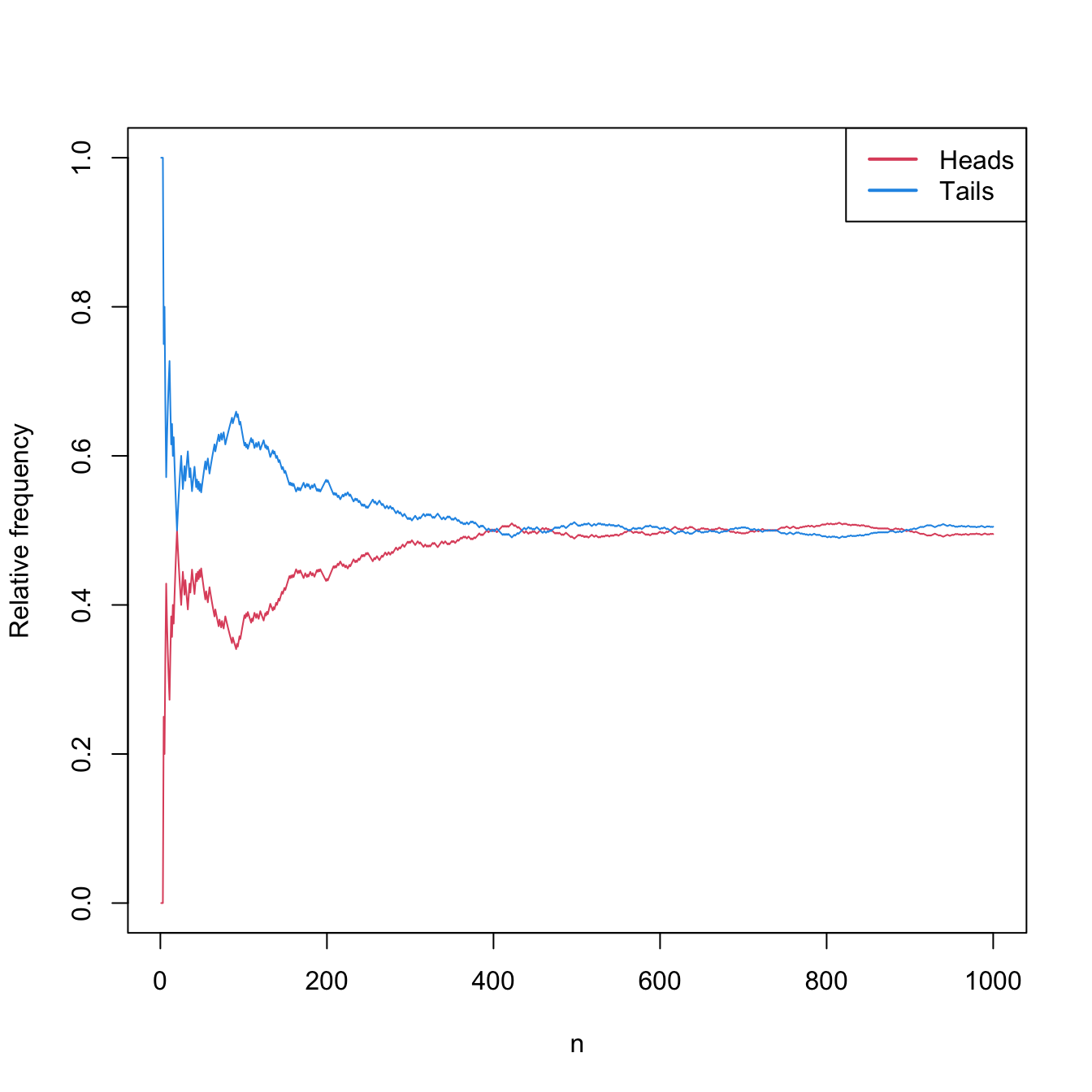

$Convergence of the relative frequencies of “heads” and “tails” to $0.5$ as the number of random experiments $n$ grows.$

Figure 1.2: Convergence of the relative frequencies of “heads” and “tails” to $0.5$ as the number of random experiments $n$ grows.

Measuring the number of car accidents for $n$ independent hours in Spain (simulated data). Table 1.2 and Figure 1.3 show the convergence of the relative frequencies of the experiment.

Table 1.2: Relative frequencies of car accidents in Spain for $n$ hours.
$n$	$0$	$1$	$2$	$3$	$4$	$5$	$\geq 6$
10	0.000	0.000	0.300	0.300	0.100	0.100	0.200
20	0.000	0.000	0.200	0.200	0.100	0.100	0.400
30	0.000	0.033	0.267	0.133	0.100	0.100	0.367
100	0.030	0.040	0.260	0.140	0.160	0.110	0.260
1000	0.021	0.078	0.145	0.192	0.200	0.150	0.214
10000	0.018	0.074	0.149	0.193	0.194	0.159	0.213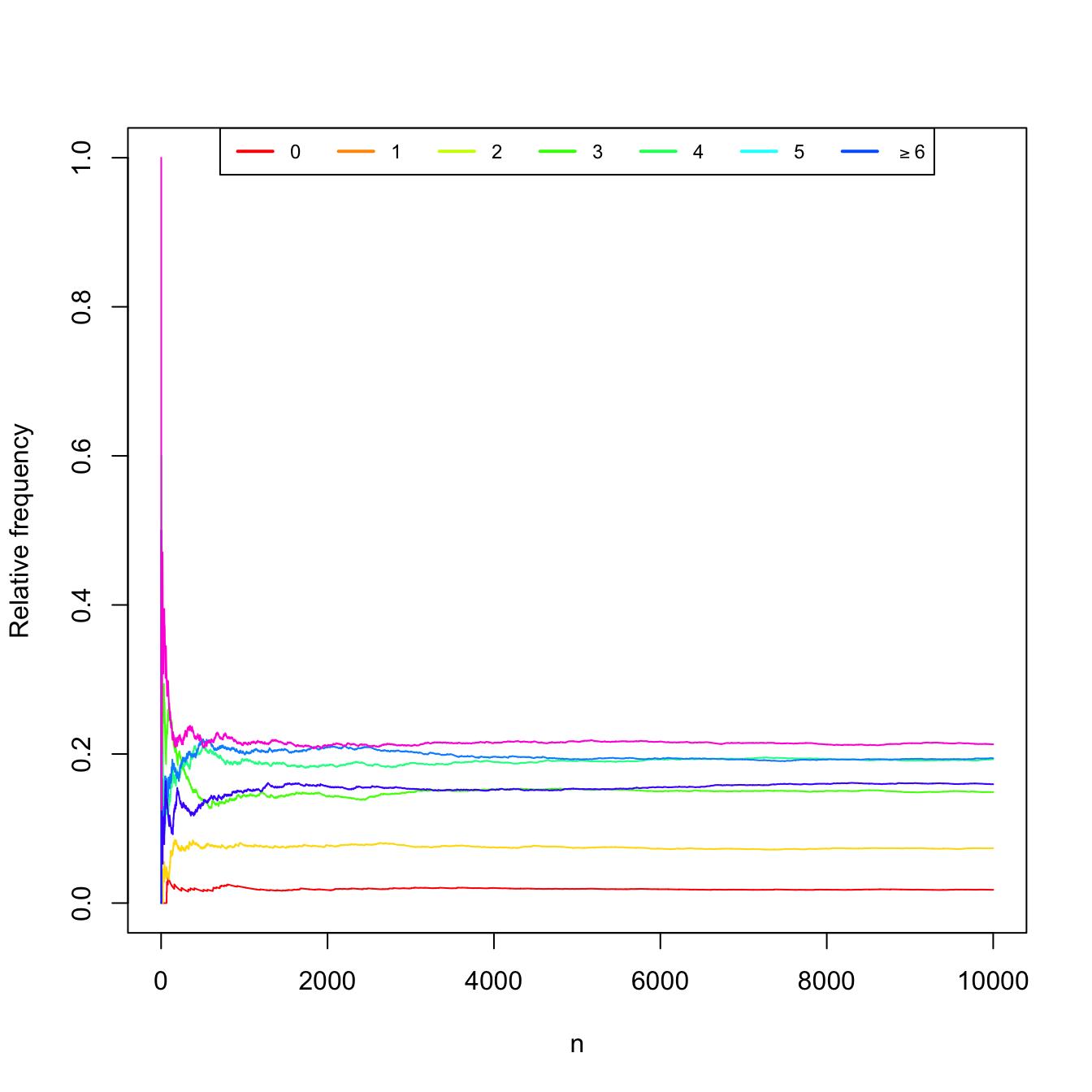

$Convergence of the relative frequencies of car accidents as the number of measured hours $n$ grows.$

Figure 1.3: Convergence of the relative frequencies of car accidents as the number of measured hours $n$ grows.

Measuring the weight (in kgs) of $n$ pedestrians between $20$ and $40$ years old. Again, Table 1.3 and Figure 1.4 show the convergence of the relative frequencies of the weight intervals.

Table 1.3: Relative frequencies of weight intervals for $n$ measured pedestrians.
$n$	$[0, 35)$	$[35, 45)$	$[45, 55)$	$[55, 65)$	$[65, \infty)$
10	0.000	0.000	0.700	0.300	0.000
20	0.000	0.100	0.700	0.200	0.000
30	0.000	0.067	0.767	0.167	0.000
100	0.000	0.220	0.670	0.110	0.000
1000	0.003	0.200	0.690	0.107	0.000
5000	0.003	0.207	0.676	0.113	0.001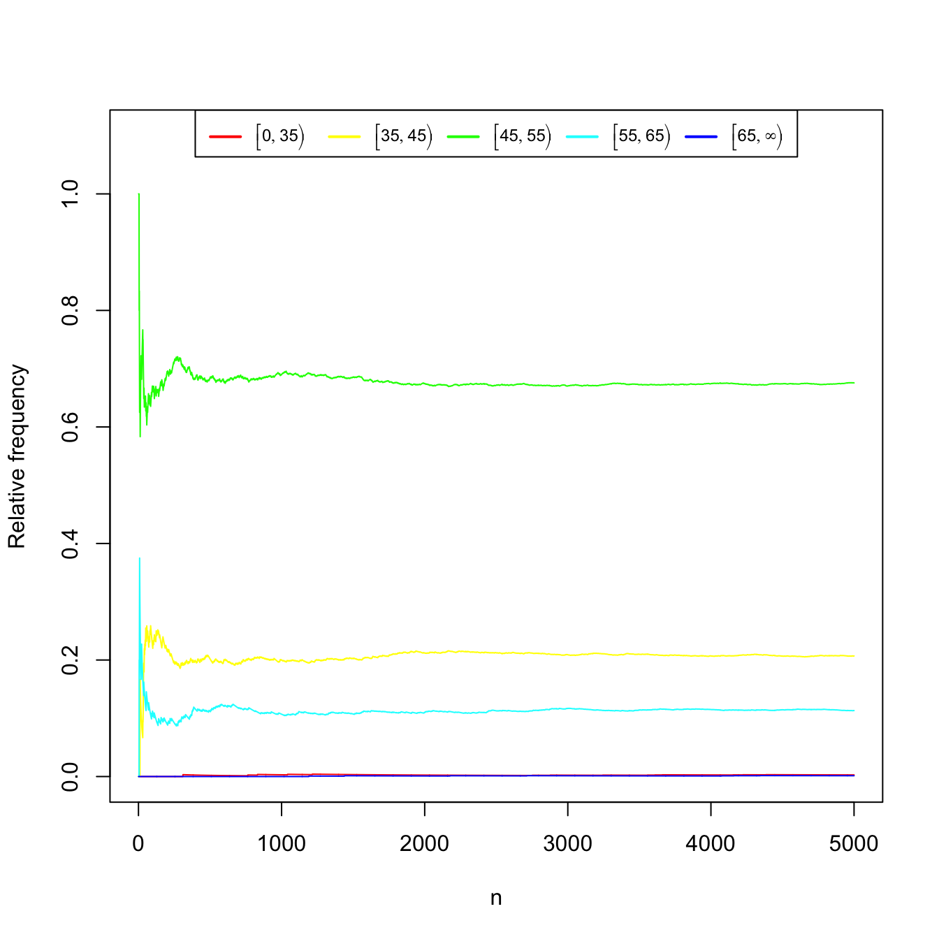

$Convergence of the relative frequencies of the weight intervals as the number of measured pedestrians $n$ grows.$

Figure 1.4: Convergence of the relative frequencies of the weight intervals as the number of measured pedestrians $n$ grows.

As hinted from the previous examples, the frequentist definition of the probability of an event is the limit of the relative frequency of that event when the number of repetitions of the experiment tends to infinity.

Definition 1.7 (Frequentist definition of probability) The frequentist definition of the probability of an event $A$ is

\[\begin{align*} \mathbb{P}(A):=\lim_{n\to\infty} \frac{n_A}{n}, \end{align*}\]

where $n$ stands for the number of repetitions of the experiment and $n_A$ is the number of repetitions in which $A$ happens.

The Laplace definition of probability can be employed for experiments that have a finite number of possible outcomes, and whose results are equally likely.

Definition 1.8 (Laplace definition of probability) The Laplace definition of probability of an event $A$ is the proportion of favorable outcomes to $A,$ that is,

\[\begin{align*} \mathbb{P}(A):=\frac{\# A}{\# \Omega}, \end{align*}\]

where $\#\Omega$ is the number of possible outcomes of the experiment and $\# A$ is the number of outcomes in $A.$

Finally, the Kolmogorov axiomatic definition of probability does not establish the probability as a unique function, as the previous probability definitions do, but presents three axioms that must be satisfied by any so-called “probability function”.¹

Definition 1.9 (Kolmogorov definition of probability) Let $(\Omega,\mathcal{A})$ be a measurable space. A probability function is an application $\mathbb{P}:\mathcal{A}\rightarrow \mathbb{R}$ that satisfies the following axioms:

(Non-negativity) $\forall A\in\mathcal{A},$ $\mathbb{P}(A)\geq 0;$
(Unitarity) $\mathbb{P}(\Omega)=1;$
($\sigma$-additivity) For any sequence $A_1,A_2,\ldots$ of disjoint events ($A_i\cap A_j=\emptyset,$ $i\neq j$) of $\mathcal{A},$ it holds

\[\begin{align*} \mathbb{P}\left(\bigcup_{n=1}^{\infty} A_n\right)=\sum_{n=1}^{\infty} \mathbb{P}(A_n). \end{align*}\]

Observe that the $\sigma$-additivity property is well-defined: since $\mathcal{A}$ is a $\sigma$-algebra, then the countable union belongs to $\mathcal{A}$ also, and therefore the probability function takes as argument a proper element from $\mathcal{A}.$ For this reason the closedness property of $\mathcal{A}$ under unions, intersections, and complements is especially important.

Definition 1.10 (Probability space) A probability space is a trio $(\Omega,\mathcal{A}, \mathbb{P}),$ where $\mathbb{P}$ is a probability function defined on the measurable space $(\Omega,\mathcal{A}).$

Example 1.4 Consider the first experiment described in Example 1.1 with the measurable space $(\Omega,\mathcal{A}),$ where

\[\begin{align*} \Omega=\{\mathrm{H},\mathrm{T}\}, \quad \mathcal{A}=\{\emptyset,\{\mathrm{H}\},\{\mathrm{T}\},\Omega\}. \end{align*}\]

A probability function is $\mathbb{P}_1:\mathcal{A}\rightarrow[0,1],$ defined as

\[\begin{align*} \mathbb{P}_1(\emptyset):=0, \ \mathbb{P}_1(\{\mathrm{H}\}):=\mathbb{P}_1(\{\mathrm{T}\}):=1/2, \ \mathbb{P}_1(\Omega):=1. \end{align*}\]

It is straightforward to check that $\mathbb{P}_1$ satisfies the three definitions of probability. Consider now $\mathbb{P}_2:\mathcal{A}\rightarrow[0,1]$ defined as

\[\begin{align*} \mathbb{P}_2(\emptyset):=0, \ \mathbb{P}_2(\{\mathrm{H}\}):=p<1/2, \ \mathbb{P}_2(\{\mathrm{T}\}):=1-p, \ \mathbb{P}_2(\Omega):=1. \end{align*}\]

If the coin is fair, then $\mathbb{P}_2$ does not satisfy the frequentist definition nor the Laplace definition, since the outcomes are not equally likely. However, it does verify the Kolmogorov axiomatic definition. Several probability functions, as well as several probability spaces, are mathematically possible! But, of course, ones are more sensible than others according to the random experiment they are modeling.

Example 1.5 We can define a probability function for the second experiment of Example 1.1, with the measurable space $(\Omega,\mathcal{P}(\Omega)),$ in the following way:

For the individual outcomes, the probability is defined as

\[\begin{align*} \begin{array}{lllll} &\mathbb{P}(\{0\}):=0.018, &\mathbb{P}(\{1\}):=0.074, &\mathbb{P}(\{2\}):=0.149, \\ &\mathbb{P}(\{3\}):=0.193, &\mathbb{P}(\{4\}):=0.194, &\mathbb{P}(\{5\}):=0.159, \\ &\mathbb{P}(\{6\}):=0.106, &\mathbb{P}(\{7\}):=0.057, &\mathbb{P}(\{8\}):=0.028, \\ &\mathbb{P}(\{9\}):=0.022, &\mathbb{P}(\emptyset):=0, &\mathbb{P}(\{i\}):=0,\ \forall i>9. \end{array} \end{align*}\]

For subsets of $\Omega$ with more than one element, its probability is defined as the sum of probabilities of the individual outcomes belonging to each subset. This is, if $A=\{a_1,\ldots,a_n\},$ with $a_i\in \Omega,$ then the probability of $A$ is

\[\begin{align*} \mathbb{P}(A):=\sum_{i=1}^n \mathbb{P}(\{a_i\}). \end{align*}\]

This probability function indeed satisfies the Kolmogorov axiomatic definition.

Example 1.6 Consider a modification of the first experiment described in Example 1.1, where now $\xi=$ “Toss a coin two times”. Then,

\[\begin{align*} \Omega=\{\mathrm{HH},\mathrm{HT},\mathrm{TH},\mathrm{TT}\}. \end{align*}\]

We define

\[\begin{align*} \mathcal{A}_1=\{\emptyset,\{\mathrm{HH}\},\ldots,\{\mathrm{HH},\mathrm{HT}\},\ldots,\{\mathrm{HH},\mathrm{HT},\mathrm{TH}\},\ldots,\Omega\}=\mathcal{P}(\Omega). \end{align*}\]

Recall that the cardinality of $\mathcal{P}(\Omega)$ is $\#\mathcal{P}(\Omega)=2^{\#\Omega}.$ This can be easily checked for this example by adding how many events comprised by $0\leq k\leq4$ outcomes are possible: $\binom{4}{0}+\binom{4}{1}+\binom{4}{2}+\binom{4}{3}+\binom{4}{4}=(1+1)^4$ (Newton’s binomial). For the measurable space $(\Omega,\mathcal{A}_1),$ a probability function $\mathbb{P}:\mathcal{A}_1\rightarrow[0,1]$ can be defined as

\[\begin{align*} \mathbb{P}(\{\omega\}):=1/4,\quad \forall \omega\in\Omega. \end{align*}\]

Then, $\mathbb{P}(A)=\sum_{\omega\in A}\mathbb{P}(\{\omega\}),$ $\forall A\in\mathcal{A}_1.$ This is a valid probability that satisfies the three Kolmogorov’s axioms (and also the frequentist and Laplace definitions) and therefore $(\Omega,\mathcal{A}_1,\mathbb{P})$ is a probability space.

Another possible $\sigma$-algebra for $\xi$ is $\mathcal{A}_2=\{\emptyset,\{\mathrm{HH}\},\{\mathrm{HT,TH,TT}\},\Omega\},$ for which $\mathbb{P}$ is well-defined. Then, another perfectly valid probability space is $(\Omega,\mathcal{A}_2,\mathbb{P}).$ This probability space would not make too much sense for modelling $\xi,$ since it assumes that the outcome $\mathrm{HT}$ is impossible, as $\mathbb{P}(\{\mathrm{HT}\})$ is not defined.

Proposition 1.1 (Basic probability results) Let $(\Omega,\mathcal{A},\mathbb{P})$ be a probability space and $A,B\in\mathcal{A}.$

Probability of the union: $\mathbb{P}(A\cup B)=\mathbb{P}(A)+\mathbb{P}(B)-\mathbb{P}(A\cap B).$
De Morgan’s rules: $\mathbb{P}(\overline{A\cup B})=\mathbb{P}(\overline{A}\cap \overline{B}),$ $\mathbb{P}(\overline{A\cap B})=\mathbb{P}(\overline{A}\cup \overline{B}).$

1.1.4 Conditional probability

Conditioning one event on another allows establishing the dependence between them via the conditional probability function.

Definition 1.11 (Conditional probability) Let $(\Omega,\mathcal{A},\mathbb{P})$ be a probability space and $A,B\in\mathcal{A}$ with $\mathbb{P}(B)>0.$ The conditional probability of $A$ given $B$ is defined as

\[\begin{align} \mathbb{P}(A|B):=\frac{\mathbb{P}(A\cap B)}{\mathbb{P}(B)}.\tag{1.1} \end{align}\]

Definition 1.12 (Independent events) Let $(\Omega,\mathcal{A},\mathbb{P})$ be a probability space and $A,B\in\mathcal{A}.$ Two events are said to be independent if $\mathbb{P}(A\cap B)=\mathbb{P}(A)\mathbb{P}(B).$

Equivalently, $A,B\in\mathcal{A}$ such that $\mathbb{P}(A),\mathbb{P}(B)>0$ are independent if $\mathbb{P}(A|B)=\mathbb{P}(A)$ or $\mathbb{P}(B|A)=\mathbb{P}(B)$ (i.e., knowing one event does not affect the probability of the other). Computing probabilities of intersections, if the events are independent, is trivial. The following results are useful for working with conditional probabilities.

Proposition 1.2 (Basic conditional probability results) Let $(\Omega,\mathcal{A},\mathbb{P})$ be a probability space.

Law of total probability: If $A_1,\ldots,A_k$ is a partition of $\Omega$ (i.e., $\Omega=\cup_{i=1}^kA_i$ and $A_i\cap A_j=\emptyset$ for $i\neq j$) that belongs to $\mathcal{A},$ $\mathbb{P}(A_i)>0$ for $i=1,\ldots,k,$ and $B\in\mathcal{A},$ then \[\begin{align*} \mathbb{P}(B)=\sum_{i=1}^k\mathbb{P}(B|A_i)\mathbb{P}(A_i). \end{align*}\]
Bayes’ theorem:² If $A_1,\ldots,A_k$ is a partition of $\Omega$ that belongs to $\mathcal{A},$ $\mathbb{P}(A_i)>0$ for $i=1,\ldots,k,$ and $B\in\mathcal{A}$ is such that $\mathbb{P}(B)>0,$ then \[\begin{align*} \mathbb{P}(A_i|B)=\frac{\mathbb{P}(B|A_i)\mathbb{P}(A_i)}{\sum_{j=1}^k\mathbb{P}(B|A_j)\mathbb{P}(A_j)}. \end{align*}\]

Proving the previous results is not difficult. Also, learning how to do it is a good way of always remembering them.

Note this definition frees the mathematical meaning of probability from the “tyranny” of the random experiment by abstracting the concept of probability.↩︎
“Theorem” might be an overstatement for this result, which is obtained from two lines of mathematics. That’s why it is many times known as the Bayes formula.↩︎