3.7 Robust estimators
An estimator \(\hat{\theta}\) of the parameter \(\theta\) associated to a rv with pdf \(f(\cdot;\theta)\) is robust if it preserves good properties (small bias and variance) even if the model suffers from small contamination, that is, if the assumed density \(f(\cdot;\theta)\) is just an approximation of the true density due to the presence of observations coming from other distributions.
The theory of statistical robustness is deep and has a broad toolbox of methods aimed for different contexts. This section just provides some ideas for robust estimation of the mean \(\mu\) and the standard deviation \(\sigma\) of a population. For that, we consider the following widely-used contamination model for \(f(\cdot;\theta)\):
\[\begin{align*} f(x;\theta,\varepsilon,g):=(1-\varepsilon)f(x;\theta)+\varepsilon g(x), \quad x\in \mathbb{R}, \end{align*}\]
for a small \(0<\varepsilon<0.5\) and an arbitrary pdf \(g.\) The model features a mixture of the signal pdf, \(f(\cdot;\theta),\) and the contamination pdf, \(g.\) The percentage of contamination is \(100\varepsilon\%.\)
The first example shows that the sample mean is not robust for this kind of contamination.
Example 3.33 (\(\bar{X}\) is not robust for \(\mu\)) Let \(f(\cdot;\theta)\) be the pdf of a \(\mathcal{N}(\theta,\sigma^2)\) and \((X_1,\ldots,X_n)\) a srs of that distribution. In absence of contamination, we know that the variance of the sample mean is \(\mathbb{V}\mathrm{ar}_\theta(\bar{X})=\sigma^2/n.\) It is an efficient estimator (Exercise 3.22). However, if we now contaminate with the pdf \(g\) of a \(\mathcal{N}(\theta, c\sigma^2),\) where \(c>0\) is a constant, then the variance of the sample mean \(\bar{X}\) under \(f(x;\theta,\varepsilon,c)\) becomes
\[\begin{align*} \mathbb{V}\mathrm{ar}_{\theta,\varepsilon,c}(\bar{X})=(1-\varepsilon)\sigma^2/n+\varepsilon c^2\sigma^2/n=(\sigma^2/n)(1+\varepsilon [c^2-1]). \end{align*}\]
Therefore, the relative variance increment under contamination is
\[\begin{align*} \frac{\mathbb{V}\mathrm{ar}_{\theta,\varepsilon,c}(\bar{X})}{\mathbb{V}\mathrm{ar}_\theta(\bar{X})}=1+\varepsilon [c^2-1]. \end{align*}\]
For \(c=5\) and \(\varepsilon=0.01,\) the ratio is \(1.24.\) In addition, \(\lim_{c\to\infty} \mathbb{V}\mathrm{ar}_{\theta,\varepsilon,c}(\bar{X})=\infty,\) for all \(\varepsilon>0.\) Therefore, \(\bar{X}\) is not robust.
The concept of outlier is intimately related with robustness. Outliers are “abnormal” observations in the sample that seem very unlikely for the assumed distribution model or are remarkably different from the rest of sample observations.41 Outliers can be originated by measurement errors, exceptional circumstances, changes in the data generating process, etc.
There are two main approaches for preventing outliers or contamination to undermine the estimation of \(\theta\):
- Detect the outliers through a diagnosis of the model fit and re-estimate the model once the outliers have been removed.
- Employ a robust estimator.
The first approach is the traditional one and is still popular due to its simplicity. Besides, it allows using non-robust efficient estimators that tend to be simpler to compute, provided the data has been cleared adequately. However, robust estimators may be needed even when performing the first approach, as the following example illustrates.
A simple rule to detect outliers in a normal population is to flag as outliers the observations that lie further away than \(3\sigma\) from the mean \(\mu,\) since those observations are highly extreme. Since their probability is \(0.0027,\) we expect to flag as an outlier \(1\) out of \(371\) observations if the data comes from a perfectly normal population. However, applying this procedure entails estimating first \(\mu\) and \(\sigma\) from the data. But the conventional estimators, the sample mean and variance, are also very sensitive to outliers, and therefore their estimates may hide the existence of outliers. Therefore, it is better to rely on a robust estimator, which brings us back to the second approach.
The next definition introduces a simple measure of the robustness of an estimator.
Definition 3.14 (Finite-sample breakdown point) For a sample realization \(\boldsymbol{x}=(x_1,\ldots,x_n)'\) and an integer \(m\) with \(1\leq m\leq n,\) define the set of samples that differ from \(\boldsymbol{x}\) in \(m\) observations as
\[\begin{align*} U_m({\boldsymbol{x}}):=\{\boldsymbol{y}=(y_1,\ldots,y_n)'\in\mathbb{R}^n : |\{i: x_i\neq y_i\}|=m\}. \end{align*}\]
The maximum change of an estimator \(\hat{\theta}\) when \(m\) observations are contaminated is
\[\begin{align*} A(\boldsymbol{x},m):=\sup_{\boldsymbol{y}\in U_m({\boldsymbol{x}})}|\hat{\theta}(\boldsymbol{y})-\hat{\theta}(\boldsymbol{x})| \end{align*}\]
and the breakdown point of \(\hat{\theta}\) for \(\boldsymbol{x}\) is
\[\begin{align*} \max\left\{\frac{m}{n}:A(\boldsymbol{x},m)<\infty\right\}. \end{align*}\]
The breakdown point of an estimator \(\hat{\theta}\) can be interpreted as the maximum fraction of the sample that can be changed without modifying the value of \(\hat{\theta}\) to an arbitrarily large value.
Example 3.34 It can be seen that:
- The breakdown point of the sample mean is \(0.\)
- The breakdown point of the sample median is \(\lfloor n/2\rfloor/n,\) with \(\lfloor n/2\rfloor/n\to0.5\) as \(n\to\infty.\)
- The breakdown point of the sample variance (and of the standard deviation) is \(0.\)
The so-called trimmed means defined below form a popular class of robust estimators for \(\mu\) that generalizes the mean (and median) in a very intuitive way.
Definition 3.15 (Trimmed mean) Let \((X_1,\ldots, X_n)\) be a sample. The \(\alpha\)-trimmed mean at level \(0\leq \alpha\leq 0.5\) is defined as
\[\begin{align*} T_{\alpha}:=\frac{1}{n-2m(\alpha)}\sum_{i=m(\alpha)+1}^{n-m(\alpha)}X_{(i)} \end{align*}\]
where \(m(\alpha):=\lfloor n\cdot \alpha\rfloor\) is the number of trimmed observations at each extreme and \((X_{(1)},\ldots, X_{(n)})\) is the ordered sample such that \(X_{(1)}\leq\cdots\leq X_{(n)}.\)
Observe that \(\alpha=0\) corresponds to the sample mean and \(\alpha=0.5\) to the sample median. The next result reveals that the breakdown point of the trimmed mean is approximately equal to \(\alpha>0,\) which is larger than that of the sample mean. Of course, this gain in robustness is at the expense of a moderate loss of efficiency in the form of an increased variance, which in a normal population is about a \(6\%\) increment when \(\alpha=0.10.\)
Proposition 3.1 (Properties of the trimmed mean)
- For symmetric distributions, \(T_{\alpha}\) is unbiased for \(\mu.\)
- The breakdown point of \(T_{\alpha}\) is \(m(\alpha)/n,\) with \(m(\alpha)/n\to\alpha\) as \(n\to\infty.\)
- For \(X\sim \mathcal{N}(\mu,\sigma^2),\) \(\mathbb{V}\mathrm{ar}(T_{0.1})\approx1.06\cdot \sigma^2/n\) for large \(n.\)
Another well-known class of robust estimators for the population mean is the class of \(M\)-estimators.
Definition 3.16 (\(M\)-estimator for \(\mu\)) An \(M\)-estimator for \(\mu\) based on the sample \((X_1,\ldots,X_n)\) is a statistic
\[\begin{align} \tilde{\mu}:=\arg \min_{m\in\mathbb{R}} \sum_{i=1}^n \rho\left(\frac{X_i-m}{\hat{s}}\right),\tag{3.10} \end{align}\]
where \(\hat{s}\) is a robust estimator of the standard deviation (such that \(\tilde{\mu}\) is scale-invariant) and \(\rho\) is the objective function, which satisfies the following properties:
- \(\rho\) is nonnegative: \(\rho(x)\geq 0,\) \(\forall x\in\mathbb{R}.\)
- \(\rho(0)=0.\)
- \(\rho\) is symmetric: \(\rho(x)=\rho(-x),\) \(\forall x\in\mathbb{R}.\)
- \(\rho\) is monotone nondecreasing: \(x\leq x'\implies \rho(x)\leq \rho(x'),\) \(\forall x,x'\in\mathbb{R}.\)
Example 3.35 The sample mean is the least squares estimator of the mean, that is, it minimizes
\[\begin{align*} \bar{X}=\arg\min_{m\in\mathbb{R}} \sum_{i=1}^n (X_i-m)^2 \end{align*}\]
and therefore is an \(M\)-estimator with \(\rho(x)=x^2.\)
Analogously, the sample median minimizes the sum of absolute distances
\[\begin{align*} \arg\min_{m\in\mathbb{R}} \sum_{i=1}^n |X_i-m| \end{align*}\]
and hence is an \(M\)-estimator with \(\rho(x)=|x|.\)
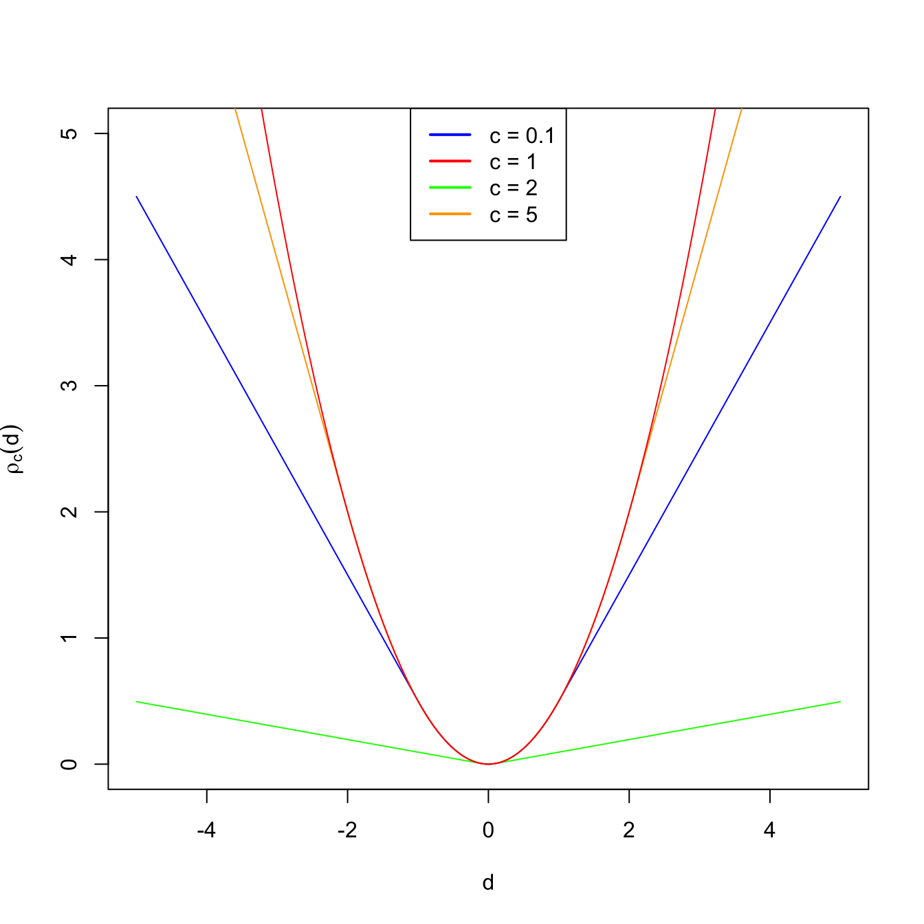
Figure 3.5: Huber’s rho function for different values of \(c\).
A popular objective function is Huber’s rho function:
\[\begin{align*} \rho_c(d)=\begin{cases} 0.5d^2 & \text{if} \ |d|\leq c,\\ c|d|-0.5c^2 & \text{if} \ |d|>c, \end{cases} \end{align*}\]
for a constant \(c>0.\) For small distances, \(\rho_c\) employs quadratic distances, as in the case of the sample mean. For large distances (that are more influential), it employs absolute distances, as the sample median does. Therefore, setting \(c\to\infty\) yields the sample mean in (3.10) and using \(c\to0\) gives the median. As with trimmed means, we therefore have an interpolation between mean (non-robust) and median (robust) that is controlled by one parameter.
Finally, a robust alternative for estimating \(\sigma\) is the median absolute deviation.
Definition 3.17 (Median absolute deviation) The Median Absolute Deviation (MAD) of a sample \((X_1,\ldots,X_n)\) is defined as
\[\begin{align*} \text{MAD}(X_1,\ldots,X_n):=c\cdot \mathrm{med}\{|X_1-\mathrm{med}\{X_1,\ldots,X_n\}|,\ldots,|X_n-\mathrm{med}\{X_1,\ldots,X_n\}|\}, \end{align*}\]
where \(\mathrm{med}\{X_1,\ldots,X_n\}\) stands for the median of the sample and \(c\) corrects the MAD such that it is centered for \(\sigma\) in normal populations:
\[\begin{align*} \mathbb{P}(|X-\mu|\le \sigma/c)=0.5\iff c=1/\Phi(0.75)\approx 1.48. \end{align*}\]
The concept of outlier is subjective, although there are several mathematical definitions of outliers.↩︎