5.1 The pivotal quantity method

Definition 5.1 (Confidence interval) Let $X$ be a rv with induced probability $\mathbb{P}(\cdot;\theta),$ $\theta\in \Theta,$ where $\Theta\subset \mathbb{R}.$ Let $(X_1,\ldots,X_n)$ be a srs of $X.$ Let $T_1=T_1(X_1,\ldots,X_n)$ and $T_2=T_2(X_1,\ldots,X_n)$ be two unidimensional statistics such that

\[\begin{align} \mathbb{P}(T_1\leq \theta\leq T_2;\theta)\geq 1-\alpha, \quad \forall \theta\in\Theta.\tag{5.1} \end{align}\]

Then, the interval $\mathrm{CI}_{1-\alpha}(\theta):=[T_1(x_1,\ldots,x_n),T_2(x_1,\ldots,x_n)]$ obtained for any sample realization $(x_1,\ldots,x_n)$ is referred to as a confidence interval for $\theta$ at the confidence level $1-\alpha$.

The value $\alpha$ is denoted as the significance level. $T_1$ and $T_2$ are known as the inferior and the superior limits of the confidence interval for $\theta,$ respectively. Sometimes the interest lies in only one of these limits.

Definition 5.2 (Pivot) A pivot $Z(\theta)\equiv Z(\theta;X_1,\ldots,X_n)$ is a function of the sample $(X_1,\ldots,X_n)$ and the unknown parameter $\theta$ that is bijective in $\theta$ and has a completely known distribution.

The pivotal quantity method for obtaining a confidence interval consists in, once fixed the significance level $\alpha$ desired to satisfy (5.1), find a pivot $Z(\theta)$ and, using the pivot’s distribution, select two constants $c_1$ and $c_2$ such that

\[\begin{align} \mathbb{P}_Z(c_1\leq Z(\theta)\leq c_2)\geq 1-\alpha. \tag{5.2} \end{align}\]

Then, solving⁶⁰ for $\theta$ in the inequalities we obtain an equivalent probability to (5.2). If $\theta\mapsto Z(\theta)$ is increasing, then (5.2) equals

\[\begin{align*} \mathbb{P}_Z(Z^{-1}(c_1)\leq \theta \leq Z^{-1}(c_2))\geq 1-\alpha, \end{align*}\]

so $T_1=Z^{-1}(c_1)$ and $T_2=Z^{-1}(c_2).$ If $Z$ is decreasing, then $T_1=Z^{-1}(c_2)$ and $T_2=Z^{-1}(c_1).$ In any case, $[T_1,T_2]$ is a confidence interval for $\theta$ at confidence level $1-\alpha.$

Usually, the pivot $Z(\theta)$ can be constructed from an estimator $\hat{\theta}$ of $\theta.$ Assume that making a transformation of the estimator $\hat{\theta}$ that involves $\theta$ we obtain $\hat{\theta}'.$ If the distribution of $\hat{\theta}'$ does not depend on $\theta,$ then we have that $\hat{\theta}'$ is a pivot for $\theta.$ For this process to work, it is key that $\hat{\theta}$ has a known distribution⁶¹ that depends on $\theta$: otherwise the constants $c_1$ and $c_2$ in (5.2) are not computable in practice.

The interpretation of confidence intervals has to be done with a certain care. Notice that in (5.1) the probability operator refers to the randomness of the interval $[T_1,T_2].$ This random confidence interval is said to contain the unknown parameter $\theta$ “with a probability of $1-\alpha$”. Yet, in reality, either $\theta$ belongs or does not belong to the interval, which seems contradictory. The previous quoted statement has to be understood in the frequentist sense of probability:⁶² when the confidence intervals are computed independently over an increasing number of samples,⁶³ the relative frequency of the event “$\theta\in\mathrm{CI}_{1-\alpha}(\theta)$” converges to $1-\alpha.$ For example, suppose you have 100 samples generated according to a certain distribution model depending on $\theta.$ If you compute $\mathrm{CI}_{1-\alpha}(\theta)$ for each of the samples, then in approximately $100(1-\alpha)$ of the samples the true parameter $\theta$ would be actually inside the random confidence interval. This is illustrated in Figure 5.2.

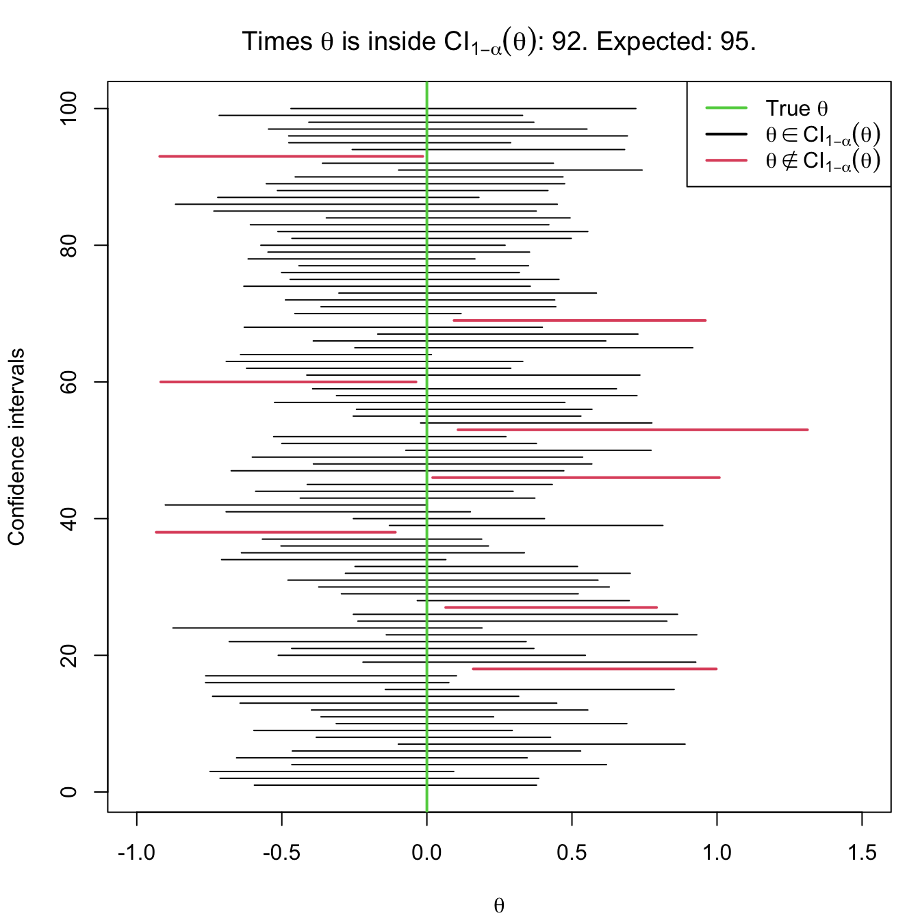
$Illustration of the randomness of the confidence interval for $\theta$ at the $1-\alpha$ confidence. The plot shows 100 random confidence intervals for $\theta,$ computed from 100 random samples generated by the same distribution model (depending on $\theta$).$

Figure 5.2: Illustration of the randomness of the confidence interval for $\theta$ at the $1-\alpha$ confidence. The plot shows 100 random confidence intervals for $\theta,$ computed from 100 random samples generated by the same distribution model (depending on $\theta$).

Example 5.1 Assume that we have a single observation $X$ of a $\mathrm{Exp}(1/\theta)$ rv. Employ $X$ to construct a confidence interval for $\theta$ with a confidence level $0.90.$

We have a srs of size one and we need to find a pivot for $\theta,$ that is, a function of $X$ and $\theta$ whose distribution is completely known. The pdf and the mgf of $X$ are given by

\[\begin{align*} f_X(x)=\frac{1}{\theta}e^{-x/\theta}, \quad x>0, \quad m_X(s)=(1-\theta s)^{-1}. \end{align*}\]

Then, taking $Z=X/\theta,$ the mgf of $Z$ is

\[\begin{align*} m_Z(s)=m_{X/\theta}(s)=m_X(s/\theta)=\left(1-\theta\frac{s}{\theta}\right)^{-1}=(1-s)^{-1}. \end{align*}\]

Therefore, $m_Z$ does not depend on $\theta$ and, in addition, is the mgf of a rv $\mathrm{Exp}(1)$ with pdf

\[\begin{align*} f_Z(z)=e^{-z}, \quad z> 0. \end{align*}\]

Then, we need to find two constants $c_1$ and $c_2$ such that

\[\begin{align*} \mathbb{P}(c_1\leq Z\leq c_2)\geq 0.90. \end{align*}\]

We know that

\[\begin{align*} \mathbb{P}(Z\leq c_1)&=\int_{0}^{c_1} e^{-z}\,\mathrm{d}z=1-e^{-c_1},\\ \mathbb{P}(Z\geq c_2)&=\int_{c_2}^{\infty} e^{-z}\,\mathrm{d}z=e^{-c_2}. \end{align*}\]

Splitting the probability $0.10$ evenly in two,⁶⁴ then

\[\begin{align*} 1-e^{-c_1}=0.05, \quad e^{-c_2}=0.05. \end{align*}\]

Solving for the $c_1$ and $c_2,$ we obtain

\[\begin{align*} c_1=-\log(0.95)\approx0.051,\quad c_2=-\log(0.05)\approx2.996. \end{align*}\]

Therefore, it is verified

\[\begin{align*} \mathbb{P}(c_1\leq X/\theta\leq c_2)= 0.9. \end{align*}\]

Solving $\theta$ from the inequalities, we have

\[\begin{align*} \mathbb{P}(X/2.996\leq \theta\leq X/0.051)\approx 0.9, \end{align*}\]

so the confidence interval for $\theta$ at significance level $0.10$ is

\[\begin{align*} \mathrm{CI}_{0.90}(\theta)\approx[X/2.996,X/0.051]. \end{align*}\]

Therefore, it is key that $Z$ is bijective in $\theta$ to be invertible.↩︎
If the distribution of $\hat{\theta}$ is only known asymptotically, then one can build an asymptotic confidence interval through the pivot method; see Section 5.4.↩︎
See Definition 1.7.↩︎
For fixed sample size! The $n$ does not change. What is repeated is the extraction of new samples.↩︎
Other splittings are possible.↩︎