3.1 Unbiased estimators

Definition 3.2 (Unbiased estimator) Given an estimator \(\hat{\theta}\) of a parameter \(\theta,\) the quantity \(\mathrm{Bias}\big[\hat{\theta}\big]:=\mathbb{E}\big[\hat{\theta}\big]-\theta\) is the bias of the estimator \(\hat{\theta}.\) The estimator \(\hat{\theta}\) is unbiased if its bias is zero, i.e., if \(\mathbb{E}\big[\hat{\theta}\big]=\theta.\)

Example 3.2 We saw in (2.5) and (2.6) that the sample variance \(S^2\) was not an unbiased estimator of \(\sigma^2,\) whereas the sample quasivariance \(S'^2\) was unbiased. From Theorem 2.2 we can see, from an alternative approach based on assuming normality, that \(S^2\) is indeed biased. On one hand,

\[\begin{align} \mathbb{E}\left[\frac{nS^2}{\sigma^2}\right]=\mathbb{E}\left[\frac{(n-1)S'^2}{\sigma^2}\right]=\mathbb{E}\left[\chi_{n-1}^2\right]=n-1 \tag{3.1} \end{align}\]

and, on the other,

\[\begin{align} \mathbb{E}\left[\frac{nS^2}{\sigma^2}\right]=\frac{n}{\sigma^2}\mathbb{E}[S^2]. \tag{3.2} \end{align}\]

Therefore, equating (3.1) and (3.2) and solving for \(\mathbb{E}[S^2],\) we have

\[\begin{align*} \mathbb{E}[S^2]=\frac{n-1}{n}\,\sigma^2. \end{align*}\]

We can also see that \(S'^2\) is indeed unbiased. First, we have that

\[\begin{align*} \mathbb{E}\left[\frac{(n-1)S'^2}{\sigma^2}\right]=\frac{n-1}{\sigma^2}\mathbb{E}[S'^2]. \end{align*}\]

Then, equating this expectation with the mean of a rv \(\chi^2_{n-1},\) \(n-1,\) and solving for \(\mathbb{E}[S'^2],\) it follows that \(\mathbb{E}[S'^2]=\sigma^2.\)

Example 3.3 Let \(X\sim\mathcal{U}(0,\theta),\) that is, its pdf is \(f_X(x)=1/\theta,\) \(0<x<\theta.\) Let \((X_1,\ldots,X_n)\) be a srs of \(X.\) Let us obtain an unbiased estimator of \(\theta.\)

Since \(\theta\) is the upper bound for the sample realization, the value from the sample that is closer to \(\theta\) is \(X_{(n)},\) the maximum of the sample. Hence, we take \(\hat{\theta}:=X_{(n)}\) as an estimator of \(\theta\) and check whether it is unbiased. In order to compute its expectation, we need to obtain its pdf. We can derive it from Exercise 2.2: the cdf \(X_{(n)}\) for a srs of a rv with cdf \(F_X\) is \([F_X]^n.\)

The cdf of \(X\) for \(0< x < \theta\) is

\[\begin{align*} F_X(x)=\int_0^x f_X(t)\,\mathrm{d}t=\int_0^x \frac{1}{\theta}\,\mathrm{d}t=\frac{x}{\theta}. \end{align*}\]

Then, the full cdf is

\[\begin{align*} F_X(x)=\begin{cases} 0 & x<0,\\ x/\theta & 0\leq x<\theta,\\ 1 & x\geq \theta. \end{cases} \end{align*}\]

Consequently, the cdf of the maximum is

\[\begin{align*} F_{X_{(n)}}(x)=\begin{cases} 0 & x<0,\\ (x/\theta)^n, & 0\leq x<\theta,\\ 1, & x\geq \theta. \end{cases} \end{align*}\]

The density of \(X_{(n)}\) follows by differentiation:

\[\begin{align*} f_{X_{(n)}}(x)=\frac{n}{\theta}\left(\frac{x}{\theta}\right)^{n-1}, \quad x\in (0,\theta). \end{align*}\]

Finally, the expectation of \(\hat{\theta}=X_{(n)}\) is

\[\begin{align*} \mathbb{E}\big[\hat{\theta}\big]&=\int_0^{\theta} x \frac{n}{\theta}\left(\frac{x}{\theta}\right)^{n-1}\,\mathrm{d}x=\frac{n}{\theta^n}\int_0^{\theta} x^n\,\mathrm{d}x\\ &=\frac{n}{\theta^n}\frac{\theta^{n+1}}{n+1}=\frac{n}{n+1}\theta\neq\theta. \end{align*}\]

Therefore, \(\hat{\theta}\) is not unbiased. However, it can be readily patched as

\[\begin{align*} \hat{\theta}':=\frac{n+1}{n}X_{(n)}, \end{align*}\]

which is an unbiased estimator of \(\theta\):

\[\begin{align*} \mathbb{E}\big[\hat{\theta}'\big]=\frac{n+1}{n}\frac{n}{n+1}\theta=\theta. \end{align*}\]

Example 3.4 Let \(X\sim \mathrm{Exp}(\theta)\) and let \((X_1,\ldots,X_n)\) be a srs of such rv. Let us find an unbiased estimator for \(\theta.\)

Since \(X\sim \mathrm{Exp}(\theta),\) we know that \(\mathbb{E}[X]=1/\theta\) and hence \(\theta=1/\mathbb{E}[X].\) As \(\bar{X}\) is an unbiased estimator of \(\mathbb{E}[X],\) it is reasonable to consider \(\hat{\theta}:=1/\bar{X}\) as an estimator of \(\theta.\) Checking whether it is unbiased requires knowing the pdf of \(\hat{\theta}.\) Since \(\mathrm{Exp}(\theta)\stackrel{d}{=}\Gamma(1,1/\theta),\) by the additive property of the gamma (see Exercise 1.21):

\[\begin{align*} T=\sum_{i=1}^n X_i\sim \Gamma\left(n,1/\theta\right), \end{align*}\]

with pdf

\[\begin{align*} f_T(t)=\frac{1}{(n-1)!} \theta^n t^{n-1} e^{-\theta t}, \quad t>0. \end{align*}\]

Then, the expectation of the estimator \(\hat{\theta}=n/T=1/\bar{X}\) is given by

\[\begin{align*} \mathbb{E}\big[\hat{\theta}\big]&=\int_0^{\infty} \frac{n}{t}\frac{1}{(n-1)!} \theta^n t^{n-1} e^{-\theta t}\,\mathrm{d}t\\ &=\frac{n \theta}{n-1}\int_0^{\infty}\frac{1}{(n-2)!} \theta^{n-1} t^{(n-1)-1} e^{-\theta t}\,\mathrm{d}t\\ &=\frac{n}{n-1} \theta. \end{align*}\]

Therefore, counterintuitively, \(\hat{\theta}\) is not unbiased for \(\theta.\) However, the corrected estimator

\[\begin{align*} \hat{\theta}'=\frac{n-1}{n}\frac{1}{\bar{X}} \end{align*}\]

is unbiased.

In the previous example we have seen that, even if \(\bar{X}\) is unbiased for \(\mathbb{E}[X],\) \(1/\bar{X}\) is biased for \(1/\mathbb{E}[X].\) This illustrates that, even if \(\hat{\theta}\) is an unbiased estimator of \(\theta,\) then in general a transformation by a function \(g\) results in an estimator \(g(\hat{\theta})\) that is not unbiased for \(g(\theta).\)³²

The quantity \(\hat{\theta}-\theta\) is the estimation error, and depends on the particular value of \(\hat{\theta}\) for the observed (or realized) sample. Observe that the bias is the expected (or mean) estimation error across all the possible realizations of the sample, which does not depend on the actual realization of \(\hat{\theta}\) for a particular sample:

\[\begin{align*} \mathrm{Bias}\big[\hat{\theta}\big]=\mathbb{E}\big[\hat{\theta}\big]-\theta=\mathbb{E}\big[\hat{\theta}-\theta\big]. \end{align*}\]

If the estimation error is measured in absolute value, \(|\hat{\theta}-\theta|,\) the quantity \(\mathbb{E}\big[|\hat{\theta}-\theta|\big]\) is referred to as the mean absolute error. If the square is taken, \((\hat{\theta}-\theta)^2,\) then we obtain the so-called Mean Squared Error (MSE)

\[\begin{align*} \mathrm{MSE}\big[\hat{\theta}\big]=\mathbb{E}\big[(\hat{\theta}-\theta)^2\big]. \end{align*}\]

The MSE is mathematically more tractable than the mean absolute error, hence is usually preferred. Since the MSE gives an average of the squared estimation errors, it introduces a performance measure for comparing two estimators \(\hat{\theta}_1\) and \(\hat{\theta}_2\) of a parameter \(\theta.\) The estimator with the lowest MSE is the optimal for estimating \(\theta\) according to the MSE performance measure.

A key identity for the MSE is the following bias-variance decomposition:

\[\begin{align*} \mathrm{MSE}\big[\hat{\theta}\big]&=\mathbb{E}\big[(\hat{\theta}-\theta)^2\big]\\ &=\mathbb{E}\big[(\hat{\theta}-\mathbb{E}\big[\hat{\theta}\big]+\mathbb{E}\big[\hat{\theta}\big]-\theta)^2\big]\\ &=\mathbb{E}\big[(\hat{\theta}-\mathbb{E}\big[\hat{\theta}\big])^2\big]+\mathbb{E}\big[(\mathbb{E}[\hat{\theta}]-\theta)^2\big]+2\mathbb{E}\big[(\hat{\theta}-\mathbb{E}\big[\hat{\theta}\big])\big](\mathbb{E}\big[\hat{\theta}\big]-\theta)\\ &=\mathbb{V}\mathrm{ar}\big[\hat{\theta}\big]+(\mathbb{E}[\theta]-\theta)^2\\ &=\mathrm{Bias}^2\big[\hat{\theta}\big]+\mathbb{V}\mathrm{ar}\big[\hat{\theta}\big]. \end{align*}\]

This identity tells us that if we want to minimize the MSE, it does not suffice to find an unbiased estimator: the variance contributes to the MSE the same as the squared bias. Therefore, if we search for the optimal estimator in terms of MSE, both bias and variance must be minimized.

Figure 3.2 shows four extreme cases of the MSE decomposition: (1) low bias and low variance (ideal); (2) low bias and large variance; (3) large bias and low variance; (4) large bias and large variance (worst). The following is a good analogy of these four cases in terms of a game of darts. The bullseye is \(\theta,\) the desired target value to hit. Each dart thrown is a realization of the estimator \(\hat{\theta}.\) The case (1) represents an experienced player: his/her darts land close to the bullseye consistently. Case (2) represents a less skilled player that has high variability about the target. Cases (3) and (4) represent players that make systematic errors.

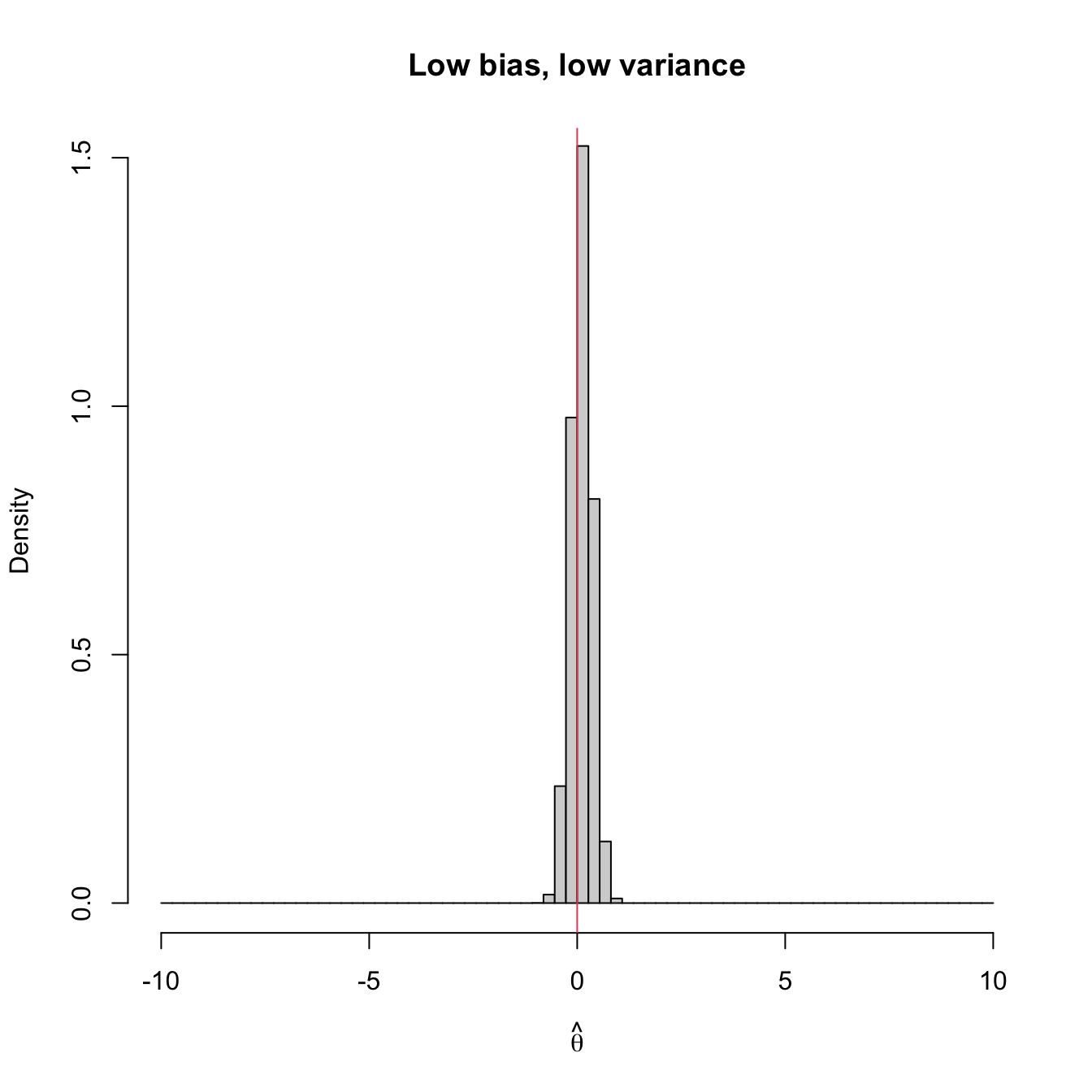
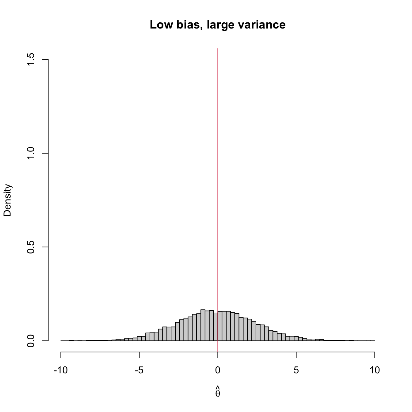
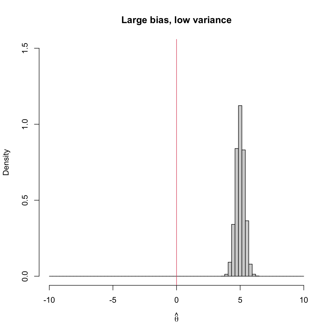
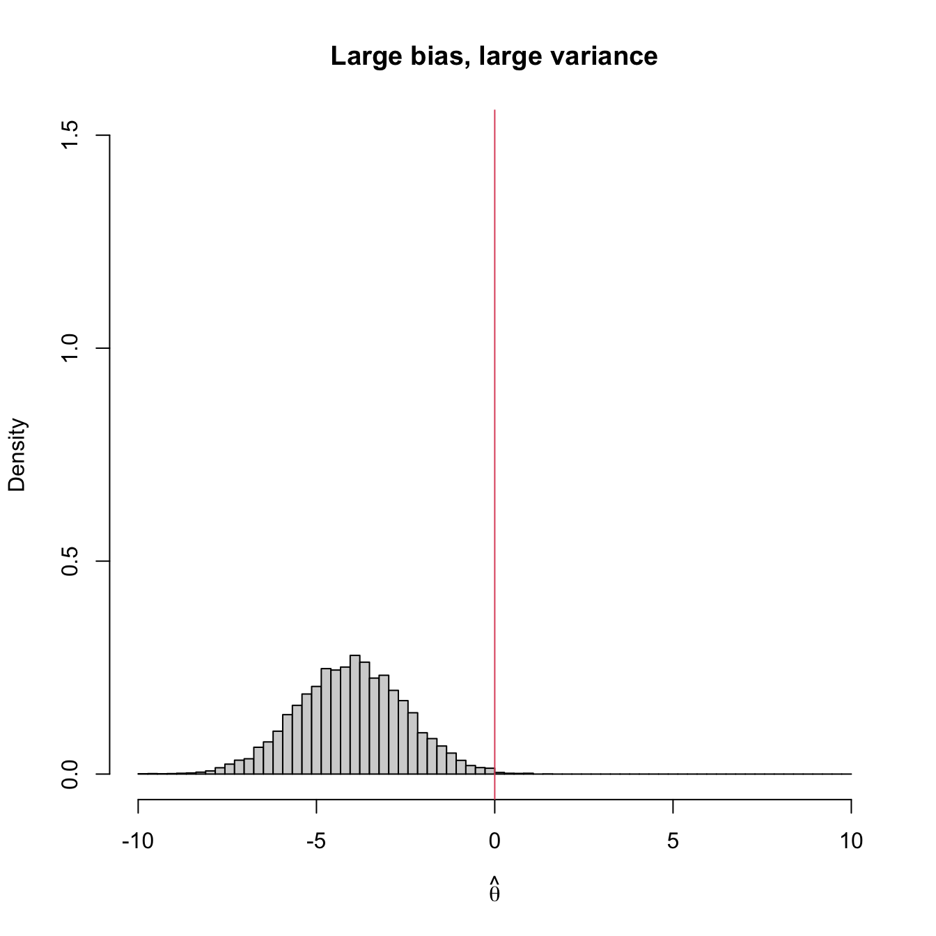
Figure 3.2: Bias and variance of an estimator \(\hat{\theta},\) represented by the positioning of its simulated distribution (histogram) with respect to the target parameter \(\theta=0\) (red vertical line).

Example 3.5 Let us compute the MSE of the sample variance \(S^2\) and the sample quasivariance \(S'^2\) when estimating the population variance \(\sigma^2\) of a normal rv (this assumption is fundamental for obtaining the expression for the variance of \(S^2\) and \(S'^2\)).

In Exercise 2.19 we saw that, for a normal population,

\[\begin{align*} \mathbb{E}[S^2]&=\frac{n-1}{n}\sigma^2, & \mathbb{V}\mathrm{ar}[S^2]&=\frac{2(n-1)}{n^2}\sigma^4,\\ \mathbb{E}[S'^2]&=\sigma^2, & \mathbb{V}\mathrm{ar}[S'^2]&=\frac{2}{n-1}\sigma^4. \end{align*}\]

Therefore, the bias of \(S^2\) is

\[\begin{align*} \mathrm{Bias}[S^2]=\frac{n-1}{n}\sigma^2-\sigma^2=-\frac{1}{n}\sigma^2<0 \end{align*}\]

and the MSE of \(S^2\) for estimating \(\sigma^2\) is

\[\begin{align*} \mathrm{MSE}[S^2]=\mathrm{Bias}^2[S^2]+\mathbb{V}\mathrm{ar}[S^2]=\frac{1}{n^2}\sigma^4+\frac{2(n-1)}{n^2}\sigma^4= \frac{2n-1}{n^2}\sigma^4. \end{align*}\]

Replicating the calculations for the sample quasivariance, we have that

\[\begin{align*} \mathrm{MSE}[S'^2]=\mathbb{V}\mathrm{ar}[S'^2]=\frac{2}{n-1}\sigma^4. \end{align*}\]

Since \(n>1,\) we have

\[\begin{align*} \frac{2}{n-1}>\frac{2n-1}{n^2} \end{align*}\]

and, as a consequence,

\[\begin{align*} \mathrm{MSE}[S'^2]>\mathrm{MSE}[S^2]. \end{align*}\]

The bottom line is clear: despite \(S'^2\) being unbiased and \(S^2\) not, for normal populations \(S^2\) has lower MSE than \(S'^2\) when estimating \(\sigma^2.\) Therefore, \(S^2\) is better than \(S'^2\) in terms of MSE for estimating \(\sigma^2\) in normal populations. This highlights that unbiased estimators are not always to be preferred in terms of the MSE!

The use of unbiased estimators is convenient when the sample size \(n\) is large, since in those cases the variance tends to be small. However, when \(n\) is small, the bias is usually very small compared with the variance, so a smaller MSE can be obtained by focusing on decreasing the variance. On the other hand, it is possible that, for a parameter and a given sample, there is no unbiased estimator, as the following example shows.

Example 3.6 The next game is presented to us. We have to pay \(6\) euros in order to participate and the payoff is \(12\) euros if we obtain two heads in two tosses of a coin with heads probability \(p.\) We receive \(0\) euros otherwise. We are allowed to perform a test toss for estimating the value of the success probability \(\theta=p^2.\)

In the coin toss we observe the value of the rv

\[\begin{align*} X_1=\begin{cases} 1 & \text{if heads},\\ 0 & \text{if tails}. \end{cases} \end{align*}\]

We know that \(X_1\sim \mathrm{Ber}(p).\) Let

\[\begin{align*} \hat{\theta}:=\begin{cases} \hat{\theta}_1 & \text{if} \ X_1=1,\\ \hat{\theta}_0 & \text{if} \ X_1=0. \end{cases} \end{align*}\]

be an estimator of \(\theta=p^2,\) where \(\hat{\theta}_0\) and \(\hat{\theta}_1\) are to be determined. Its expectation is

\[\begin{align*} \mathbb{E}\big[\hat{\theta}\big]=\hat{\theta}_1\times p+\hat{\theta}_0\times (1-p), \end{align*}\]

which is different from \(p^2\) for any estimator \(\hat{\theta}\); \(\mathbb{E}\big[\hat{\theta}\big]=p^2\) will be achieved if \(\hat{\theta}_1=p\) and \(\hat{\theta}_0=0,\) which is not allowed since \(\hat{\theta}\) can only depend on the sample and not on the unknown parameter. Therefore, for any given sample of size \(n=1\) there does not exist any unbiased estimator of \(p^2.\)

---

32. Can you think of a class of transformations for which unbiasedness is actually preserved?↩︎