2.3 The central limit theorem

The Central Limit Theorem (CLT) is a cornerstone result in statistics, if not the cornerstone result. The result states that the sampling distribution of the sample mean $\bar{X}$ of iid rv’s $X_1,\ldots,X_n$ converges to a normal distribution as $n\to\infty.$ The beauty of this result is that it holds irrespective of the original distribution of $X_1,\ldots,X_n.$

Theorem 2.5 (Central limit theorem) Let $X_1,\ldots,X_n$ be iid rv’s with expectation $\mathbb{E}[X_i]=\mu$ and variance $\mathbb{V}\mathrm{ar}[X_i]=\sigma^2<\infty.$ Then, the cdf of the rv

$$\begin{align*} U_n=\frac{\bar{X}-\mu}{\sigma/\sqrt{n}} \end{align*}$$

converges to the cdf of a $\mathcal{N}(0,1)$ as $n\to\infty.$

Remark. To denote “approximately distributed as” we will use $\cong.$ We can therefore write that, due to the CLT, $\frac{\bar{X}-\mu}{\sigma/\sqrt{n}}\cong \mathcal{N}(0,1)$ (as $n\to\infty$). Observe that this notation is different to $\sim,$ used to denote “distributed as”, or $\approx,$ used for approximations of numerical quantities.

Proof (Proof of Theorem 2.5). We compute the mgf of the rv $U_n.$ Since $X_1,\ldots,X_n$ are independent,

$$\begin{align*} M_{U_n}(s)&=\mathbb{E}\left[\exp\left\{s U_n\right\}\right]=\mathbb{E}\left[ \exp\left\{s\sum_{i=1}^n\left(\frac{X_i-\mu}{\sigma\sqrt{n}}\right) \right\}\right]\\ &=\prod_{i=1}^n \mathbb{E}\left[\exp\left\{s\, \frac{X_i -\mu}{\sigma\sqrt{n}}\right\}\right]. \end{align*}$$

Now, denoting $Z:=(X_1-\mu)/\sigma$ (this variable is standardized but it is not a standard normal variable), we have

$$\begin{align*} M_{U_n}(s)&=\left(\mathbb{E}\left[\exp\left\{\frac{s}{\sqrt{n}} Z\right\}\right]\right)^n=\left[M_Z\left(\frac{s}{\sqrt{n}}\right)\right]^n, \end{align*}$$

The rv $Z$ is such that $\mathbb{E}[Z]=0$ and $\mathbb{E}[Z^2]=1.$ We perform a second-order Taylor expansion of $M_Z(s/\sqrt{n})$ about $s=0$:

$$\begin{align*} M_Z\left(\frac{s}{\sqrt{n}}\right)=M_Z(0)+M_Z^{(1)}(0)\frac{\left(s/\sqrt{n}\right)}{1!}+M_Z^{(2)}(0)\frac{\left(s/\sqrt{n}\right)^2}{2!}+R(s/\sqrt{n}), \end{align*}$$

where $M_Z^{(k)}(0)$ is the $k$-th derivative of the mgf evaluated at $s=0$ and the remainder term $R$ is a function that satisfies

$$\begin{align*} \lim_{n\to\infty} \frac{R\left(s/\sqrt{n}\right)}{(s/\sqrt{n})^2}=0, \end{align*}$$

i.e., is contribution in the Taylor expansion is negligible in comparison with the second term $(s/\sqrt{n})^2$ when $n\to\infty.$

Since the derivatives evaluated at zero are equal to the moments (Theorem 1.1), we have:

$$\begin{align*} M_Z\left(\frac{s}{\sqrt{n}}\right) &=\mathbb{E}\left[e^0\right]+\mathbb{E}[Z]\frac{s}{\sqrt{n}}+\mathbb{E}\left[Z^2\right]\frac{s^2}{2n}+R\left(\frac{s}{\sqrt{n}}\right) \\ &=1+\frac{s^2}{2n}+R\left(\frac{s}{\sqrt{n}}\right) \\ &=1+\frac{1}{n}\left[\frac{s^2}{2}+nR\left(\frac{s}{\sqrt{n}}\right)\right]. \end{align*}$$

Now,

$$\begin{align*} \lim_{n\to\infty} M_{U_n}(s)&=\lim_{n\to\infty}\left[M_Z\left(\frac{s}{\sqrt{n}}\right)\right]^n\\ &=\lim_{n\to\infty}\left\{1+\frac{1}{n}\left[\frac{s^2}{2}+nR\left(\frac{s}{\sqrt{n}}\right)\right]\right\}^n. \end{align*}$$

In order to compute the limit, we use that, as $x\to0,$ $\log(1+x)=x+L(x)$ with remainder $L$ such that $\lim_{x\to 0} L(x)/x=0.$ Then,

$$\begin{align} \lim_{n\to\infty}nR\left(\frac{s}{\sqrt{n}}\right)&=\lim_{n\to\infty} s^2 \frac{R(s/\sqrt{n})}{(s/\sqrt{n})^2}=0,\tag{2.10}\\ \lim_{n\to\infty} nL\left(\frac{s^2}{2n}\right)&=\lim_{n\to\infty}\frac{2}{s^2}\frac{L\left(s^2/(2n)\right)}{s^2/(2n)}=0.\tag{2.11} \end{align}$$

Then, applying the logarithm and using its expansion plus (2.10) and (2.11), we have

$$\begin{align*} \lim_{n\to\infty} \log M_{U_n}(s)&=\lim_{n\to\infty}n\log\left\{1+\frac{1}{n}\left[\frac{s^2}{2}+nR\left(\frac{s}{\sqrt{n}}\right)\right]\right\}\\ &=\lim_{n\to\infty}n \left\{\frac{1}{n}\left[\frac{s^2}{2}+nR\left(\frac{s}{\sqrt{n}}\right)\right]+L\left(\frac{s^2}{2n}\right)\right\}\\ &=\frac{s^2}{2}+\lim_{n\to\infty} nR\left(\frac{s}{\sqrt{n}}\right)+\lim_{n\to\infty} nL\left(\frac{s^2}{2n}\right)\\ &=\frac{s^2}{2}. \end{align*}$$

Therefore,

$$\begin{align*} \lim_{n\to\infty}M_{U_n}(s)=e^{s^2/2}=M_{\mathcal{N}(0,1)}(s), \end{align*}$$

where $M_{\mathcal{N}(0,1)}(s)=e^{s^2/2}$ is seen in Exercise 1.18.

The application of Theorem 1.3 ends the proof.

Remark. If $X_1,\ldots,X_n$ are normal rv’s, then $U_n$ is exactly distributed as $\mathcal{N}(0,1).$ This is the exact version of the CLT.

Example 2.13 The grades in a first-year course of a given university have a mean of $\mu=6.1$ points (over $10$ points) and a standard deviation of $\sigma=1.5,$ both known from long-term records. A specific generation of $n=38$ students had a mean of $5.5$ points. Can we state that these students have a significant lower performance? Or perhaps this is a reasonable deviation from the average performance merely due to randomness? In order to answer, compute the probability that the sample mean is at most $5.5$ when $n=38.$

Let $\bar{X}$ be the sample mean of the srs of $n=38$ students grades. By the CLT we know that

$$\begin{align*} Z=\frac{\bar{X}-\mu}{\sigma/\sqrt{n}}\cong \mathcal{N}(0,1). \end{align*}$$

Then, we are interested in computing the probability

$$\begin{align*} \mathbb{P}(\bar{X}\leq 5.5)=\mathbb{P}\left(Z\leq \frac{5.5-6.1}{1.5/\sqrt{38}}\right)\approx\mathbb{P}(Z\leq -2.4658)\approx 0.0068, \end{align*}$$

which has been obtained with

pnorm(-2.4658)
## [1] 0.006835382
pnorm(5.5, mean = 6.1, sd = 1.5 / sqrt(38)) # Alternatively
## [1] 0.006836039

Observe that this probability is very small. This suggests that it is highly unlikely that this generation of students belongs to the population with mean $\mu=6.1.$ It is more likely that its true mean is smaller than $6.1$ and therefore the generation of current students has a significantly lower performance than previous generations.

Example 2.14 The random waiting time in a cash register of a supermarket is distributed according to a distribution with mean $1.5$ minutes and variance $1.$ What is the approximate probability of serving $n=100$ clients in less than $2$ hours?

If $X_i$ denotes the waiting time of the $i$-th client, then we want to compute

$$\begin{align*} \mathbb{P}\left(\sum_{i=1}^{100} X_i\leq 120\right)=\mathbb{P}\left(\bar{X}\leq 1.2\right). \end{align*}$$

As the sample size is large, the CLT entails that $\bar{X}\cong\mathcal{N}(1.5, 1/100),$ so

$$\begin{align*} \mathbb{P}\left(\bar{X}\leq 1.2\right)=\mathbb{P}\left(\frac{\bar{X}-1.5}{1/\sqrt{100}} \leq \frac{1.2-1.5}{1/\sqrt{100}}\right)\approx \mathbb{P}(Z\leq -3). \end{align*}$$

Employing pnorm() we can compute $\mathbb{P}(Z\leq -3)$ right away:

pnorm(-3)
## [1] 0.001349898

The CLT employs a type of convergence for sequences of rv’s that we precise next.

Definition 2.6 (Convergence in distribution) A sequence of rv’s $X_1,X_2,\ldots$ converges in distribution to a rv $X$ if

$$\begin{align*} \lim_{n\to\infty} F_{X_n}(x)=F_X(x), \end{align*}$$

for all the points $x\in\mathbb{R}$ where $F_X(x)$ is continuous. The convergence in distribution is denoted by

$$\begin{align*} X_n \stackrel{d}{\longrightarrow} X. \end{align*}$$

The thesis of the CLT can be rewritten in terms of this (more explicit) notation as follows:

$$\begin{align*} U_n=\frac{\bar{X}-\mu}{\sigma/\sqrt{n}}\stackrel{d}{\longrightarrow}\mathcal{N}(0,1). \end{align*}$$

This means that the cdf of $U_n,$ $F_{U_n},$ verifies that $\lim_{n\to\infty} F_{U_n}(x)=\Phi(x)$ for all $x\in\mathbb{R}.$ We can visualize how this convergence happens by plotting the cdf’s of $U_n$ for increasing values of $n$ and matching them with $\Phi,$ the cdf of a standard normal. This is done in Figures 2.8 and 2.9, where the cdf’s $F_{U_n}$ are approximated by Monte Carlo.

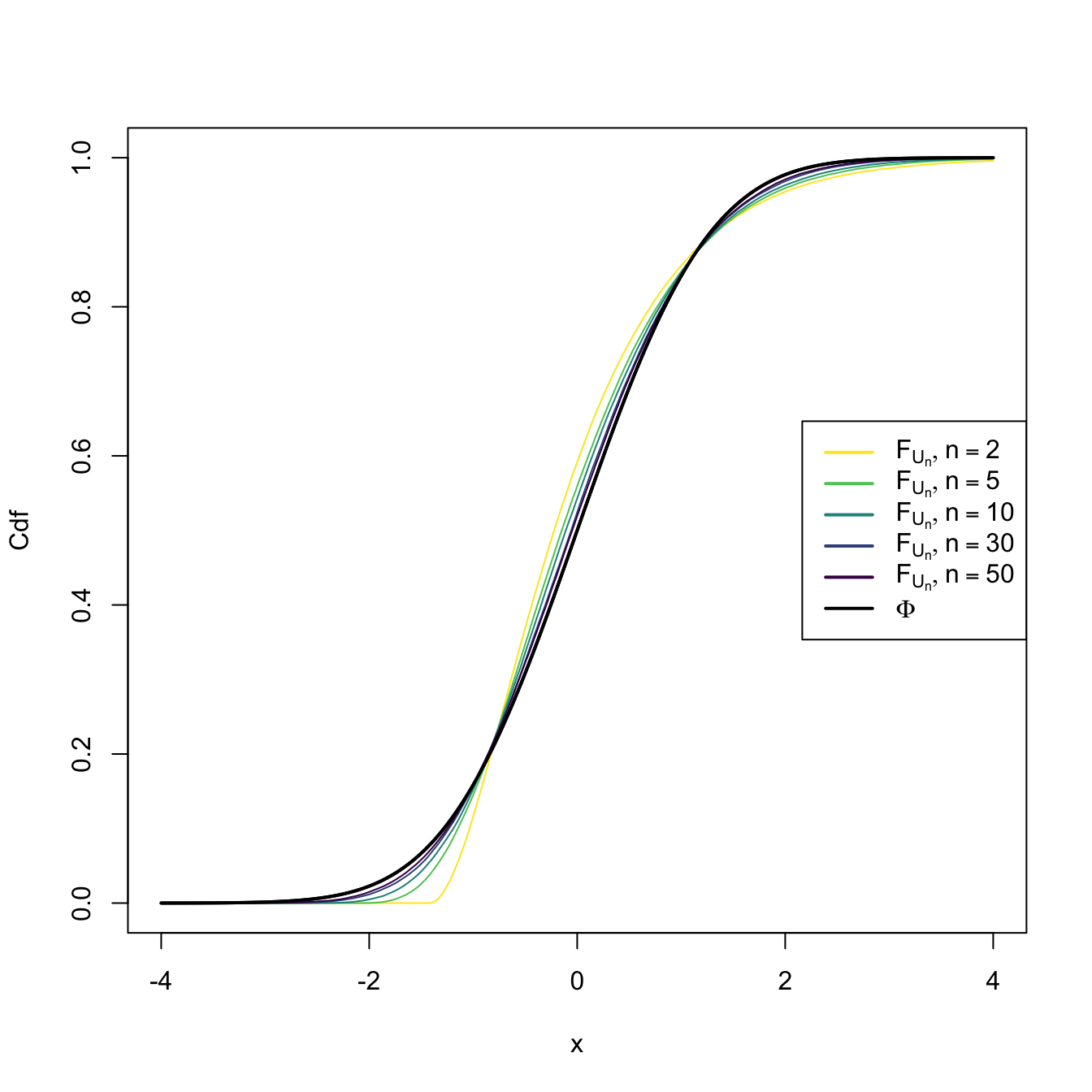
Figure 2.8: Cdf’s of $U_n=(\bar{X}-\mu)/(\sigma/\sqrt{n})$ for $X_1,\ldots,X_n\sim \mathrm{Exp}(2).$ A fast convergence of $F_{U_n}$ towards $\Phi$ appears, despite the heavy non-normality of $\mathrm{Exp}(2)$.

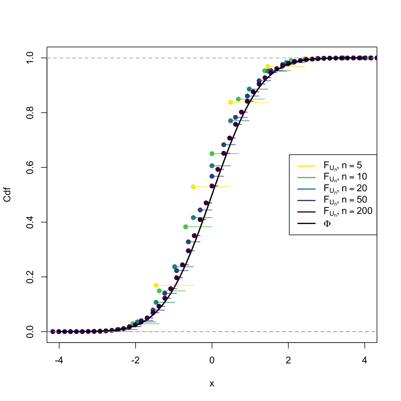
Figure 2.9: Cdf’s of $U_n=(\bar{X}-\mu)/(\sigma/\sqrt{n})$ for $X_1,\ldots,X_n\sim \mathrm{Bin}(1,p).$ The cdf’s $F_{U_n}$ are discrete for every $n,$ which makes their convergence towards $\Phi$ slower than in the continuous case.

The diagram below summarizes the available sampling distributions for the sample mean:

$$\begin{align*} \!\!\!\!\!\!\!\!(X_1,\ldots,X_n)\begin{cases} \sim \mathcal{N}(\mu,\sigma^2) & \implies \bar{X}\sim \mathcal{N}(\mu,\sigma^2/n) \\ \nsim \mathcal{N}(\mu,\sigma^2) & \begin{cases} n \;\text{ small} & \implies \text{?} \\ n \;\text{ large} & \implies \bar{X}\cong \mathcal{N}(\mu,\sigma^2/n) \end{cases} \end{cases} \end{align*}$$

The following examples provide another view on the applicability of the CLT: to approximate certain distributions for large values of their parameters.

Example 2.15 (Normal approximation to the binomial) Let $Y$ be a binomial rv of size $n\in\mathbb{N}$ and success probability $p\in[0,1]$ (see Example 1.22), denoted by $\mathrm{Bin}(n,p).$ It holds that $Y=\sum_{i=1}^n X_i,$ where $X_i\sim \mathrm{Ber}(p),$ $i=1,\ldots,n,$ with $\mathrm{Ber}(p)\stackrel{d}{=}\mathrm{Bin}(1,p)$ and $X_1,\ldots,X_n$ independent.

It is easy to see that

$$\begin{align*} \mathbb{E}[X_i]=p, \quad \mathbb{V}\mathrm{ar}[X_i]=p(1-p). \end{align*}$$

Then, applying the CLT, we have that

$$\begin{align*} \bar{X}=\frac{Y}{n}\cong \mathcal{N}\left(p,\frac{p(1-p)}{n}\right), \end{align*}$$

which implies that $\mathrm{Bin}(n,p)/n\cong \mathcal{N}\left(p,\frac{p(1-p)}{n}\right),$ or, equivalently,

$$\begin{align} \mathrm{Bin}(n,p)\cong \mathcal{N}(np,np(1-p)) \tag{2.12} \end{align}$$

as $n\to\infty.$ This approximation works well even when $n$ is not very large (i.e., $n<30$), as long as $p$ is “not very close to zero or one”, which is often translated as requiring that both $np>5$ and $np(1-p)>5$ hold.

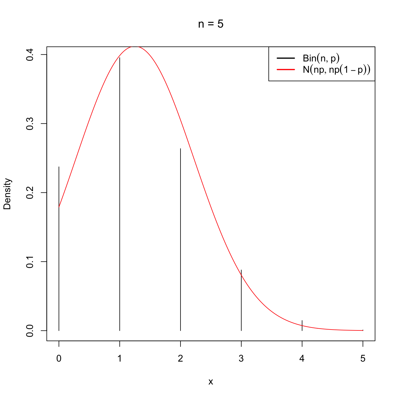
Figure 2.10: Normal approximation to the $\mathrm{Bin}(n,p)$ for $n=5$ and $n=50$ with $p=0.25$.

A continuity correction is often employed for improving the accuracy in the computation of binomial probabilities. Then, if $\tilde{Y}\sim\mathcal{N}(np,np(1-p))$ denotes the approximating rv, better approximations are obtained with

$$\begin{align*} \mathbb{P}(Y\leq m) & \approx \mathbb{P}(\tilde{Y}\leq m+0.5), \\ \mathbb{P}(Y\geq m) & \approx \mathbb{P}(\tilde{Y}\geq m-0.5), \\ \mathbb{P}(Y=m) & \approx \mathbb{P}(m-0.5\leq \tilde{Y}\leq m+0.5), \end{align*}$$

where $m\in\mathbb{N}$ and $m\leq n.$

Example 2.16 Let $Y\sim\mathrm{Bin}(25,0.4).$ Using the normal distribution, approximate the probability that $Y\leq 8$ and that $Y=8.$

Using the continuity correction, $\mathbb{P}(Y\leq 8)$ can be approximated as

$$\begin{align*} \mathbb{P}(Y\leq 8)\approx \mathbb{P}(\tilde{Y}\leq 8.5)=\mathbb{P}(\mathcal{N}(10,6)\leq 8.5). \end{align*}$$

and its actual value is

pnorm(8.5, mean = 10, sd = sqrt(6))
## [1] 0.2701457

The probability of $Y=8$ is approximated as

$$\begin{align*} \mathbb{P}(Y=8) \approx \mathbb{P}(7.5\leq \tilde{Y}\leq 8.5)=\mathbb{P}(7.5\leq \mathcal{N}(10,6)\leq 8.5) \end{align*}$$

and its actual value is

pnorm(8.5, mean = 10, sd = sqrt(6)) - pnorm(7.5, mean = 10, sd = sqrt(6))
## [1] 0.1164286

We can compare these two approximated probabilities with the exact ones

$$\begin{align*} \mathbb{P}(\mathrm{Bin}(n, p) \leq m) \text{ and } \mathbb{P}(\mathrm{Bin}(n, p) = m), \end{align*}$$

which can be computed right away with pbinom(m, size = n, prob = p) and dbinom(m, size = n, prob = p), respectively:

pbinom(8, size = 25, prob = 0.4)
## [1] 0.2735315
dbinom(8, size = 25, prob = 0.4)
## [1] 0.1199797

The normal approximation is therefore quite precise, even for $n=25.$

Example 2.17 A candidate for city major believes that he/she may win the elections if he/she obtains at least $55\%$ of the votes in district D. In addition, he/she assumes that the $50\%$ of all the voters in the city support him/her. If $n=100$ voters vote in district D (consider them as a srs of the voters of the city), what is the exact probability that the candidate wins at least the $55\%$ of the votes?

Let $Y$ be the number of voters in district D that supports the candidate. $Y$ is distributed as $\mathrm{Bin}(100,0.5)$ and we want to know the probability

$$\begin{align*} \mathbb{P}(Y/n\geq 0.55)=\mathbb{P}(Y\geq 55). \end{align*}$$

The desired probability is

$$\begin{align*} \mathbb{P}(\mathrm{Bin}(100, 0.5) \geq 55)=1-\mathbb{P}(\mathrm{Bin}(100, 0.5) < 55), \end{align*}$$

which can be computed as:

1 - pbinom(54, size = 100, prob = 0.5)
## [1] 0.1841008
pbinom(54, size = 100, prob = 0.5, lower.tail = FALSE) # Alternatively
## [1] 0.1841008

The previous value was the exact probability for a binomial. Let us see now how close the CLT approximation is. Because of the CLT,

$$\begin{align*} \mathbb{P}(Y/n\geq 0.55)\approx\mathbb{P}\left(\mathcal{N}\left(0.5, \frac{0.25}{100}\right)\geq 0.55\right) \end{align*}$$

with the actual value given by

1 - pnorm(0.55, mean = 0.5, sd = sqrt(0.25 / 100))
## [1] 0.1586553

If the continuity correction was employed, the probability is approximated to

$$\begin{align*} \mathbb{P}(Y\geq 0.55n)\approx\mathbb{P}\left(\tilde{Y}\geq 0.55n-0.5\right)=\mathbb{P}\left(\mathcal{N}\left(50, 25\right)\geq 54.5\right), \end{align*}$$

which takes the value

1 - pnorm(54.5, mean = 50, sd = sqrt(25))
## [1] 0.1840601

As seen, the continuity correction offers a significant improvement, even for $n=100$ and $p=0.5.$

Example 2.18 (Normal approximation to additive distributions) The additive property of the binomial is key for obtaining its normal approximation by the CLT seen in Example 2.15. On one hand, if $X_1,\ldots,X_n$ are $\mathrm{Bin}(1,p),$ then $n\bar{X}$ is $\mathrm{Bin}(n,p).$ On the other hand, the CLT thesis can also be expressed as

$$\begin{align} n\bar{X}\cong\mathcal{N}(n\mu,n\sigma^2) \tag{2.13} \end{align}$$

as $n\to\infty.$ Equaling both results we have the approximation (2.12).

Different additive properties are also satisfied by other distributions, as we saw in Exercise 1.20 (Poisson distribution) and Exercise 1.21 (gamma distribution). In addition, the chi-square distribution, as a particular case of the gamma, has also an additive property (Proposition 2.2) on the degrees of freedom $\nu.$ Therefore, we can obtain normal approximations for these distributions as well.

For the Poisson, we know that, if $(X_1,\ldots,X_n)$ is a srs of a $\mathrm{Pois}(\lambda),$ then

$$\begin{align} n\bar{X}=\sum_{i=1}^nX_i\sim\mathrm{Pois}(n\lambda).\tag{2.14} \end{align}$$

Since the expectation and the variance of a $\mathrm{Pois}(\lambda)$ are both equal to $\lambda,$ equaling (2.13) and (2.14) when $n\to\infty$ yields

$$\begin{align*} \mathrm{Pois}(n\lambda)\cong \mathcal{N}(n\lambda,n\lambda). \end{align*}$$

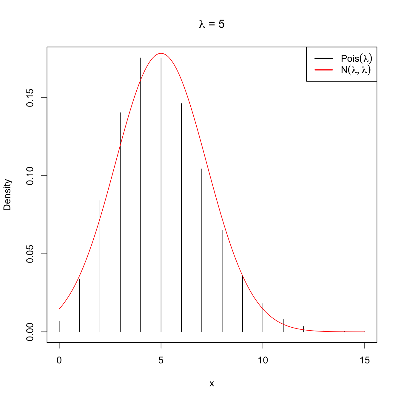
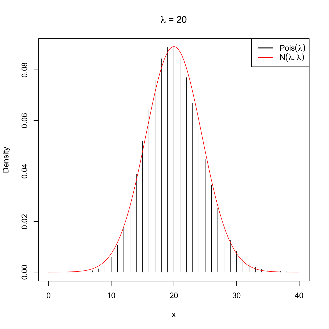
Figure 2.11: Normal approximation to the $\mathrm{Pois}(\lambda)$ for $\lambda=5$ and $\lambda=20$.

Note that this approximation is equivalent to saying that when the intensity parameter $\lambda$ tends to infinity, then $\mathrm{Pois}(\lambda)$ is approximately a $\mathcal{N}(\lambda,\lambda).$

Following similar arguments for the chi-square distribution, it is easy to see that, when $\nu\to\infty,$

$$\begin{align} \chi^2_\nu\cong \mathcal{N}(\nu,2\nu). \tag{2.15} \end{align}$$

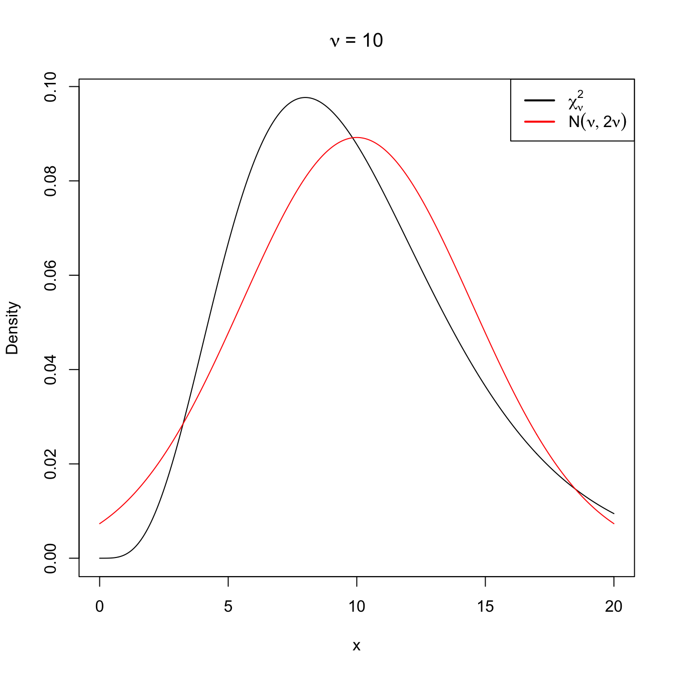
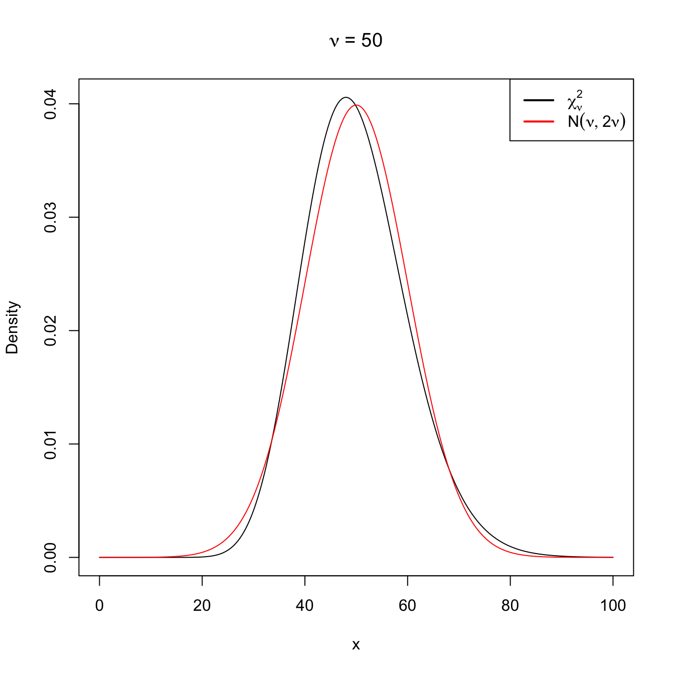
Figure 2.12: Normal approximation to the $\chi^2_\nu$ for $\nu=10$ and $\nu=50$.