5.5 Bootstrap-based confidence intervals
Each confidence interval discussed in the previous section has been obtained by a careful analysis of the sampling distribution of an estimator \(\hat{\theta}\) for the parameter \(\theta.\) Two main approaches have been used: exact results based on normal populations and asymptotic approximations via the CLT or maximum likelihood estimation. Both of them are somehow artisan approaches with important limitations. The first approach requires normal populations, which is an important practical drawback. The second approach requires the identification and exploitation of a CLT or maximum likelihood structure, which has to be done on a case-by-case basis. Neither of the approaches are, therefore, fully-automatic, despite having other important advantages, such as computational expediency and efficiency. For example, if using moment estimators \(\hat{\theta}_{\mathrm{MM}}\) because maximum likelihood is untractable, we currently do not have a form of deriving a confidence interval for \(\theta.\)
We study now a practical computational-based solution to construct confidence intervals: bootstrapping. The bootstrap motto can be summarized as
“the sample becomes the population”.
The motivation behind this motto is simple: if the sample \((X_1,\ldots,X_n)\) is large enough, then the sample is representative of the population \(X\sim F.\) Therefore, we can identify sample and population, and hence have full control on the (now discrete) population because we know it through the sample. Therefore, since we know the population, we can replicate the sample generation process in a computer in order to approximate the sampling distribution of \(\hat{\theta},\) which is key to build confidence intervals.
The previous ideas can be summarized in the following bootstrap algorithm for approximating \(\mathrm{CI}^*_{1-\alpha}(\theta),\) the bootstrap \((1-\alpha)\)-confidence interval for \(\theta,\) from a consistent estimator \(\hat{\theta}\):
Estimate \(\theta\) from the sample realization \((x_1,\ldots,x_n),\) obtaining \(\hat{\theta}(x_1,\ldots,x_n).\)70
Generate bootstrap estimators. For \(b=1,\ldots,B\):71
Approximate the bootstrap confidence interval:
- Sort the values of the bootstrap estimator: \[\begin{align*} \hat{\theta}_{(1)}^*\leq \ldots\leq \hat{\theta}_{(B)}^*. \end{align*}\]
- Extract the \(\alpha/2\) and \(1-\alpha/2\) sample quantiles: \[\begin{align*} \hat{\theta}_{(\lfloor B\,(\alpha/2)\rfloor)}^*,\quad \hat{\theta}_{(\lfloor B\,(1-\alpha/2)\rfloor)}^*. \end{align*}\]
- The \((1-\alpha)\) bootstrap confidence interval for \(\theta\) is approximated as: \[\begin{align} \widehat{\mathrm{CI}}^*_{1-\alpha}(\theta):=\left[\hat{\theta}_{(\lfloor B\,(\alpha/2)\rfloor)}^*,\hat{\theta}_{(\lfloor B\,(1-\alpha/2)\rfloor)}^*\right].\tag{5.8} \end{align}\]
Several remarks on the above bootstrap algorithm are in place:
- Observe that (5.8) is random (conditionally on the sample): it depends on the \(B\) bootstrap random samples drawn in Step 2. Thus there is an extra layer of randomness in a bootstrap confidence interval.
- The resampling in Step 2 is known as the nonparametric/ordinary/naive bootstrap resampling. No model is assumed. Another alternative is parametric bootstrap.
- The method for approximating the bootstrap confidence intervals in Step 3 is known as the percentile bootstrap. It requires large \(B\)’s for a reasonable accuracy and can be thus time-consuming. Typically, not less than \(B=1000.\) More sophisticated approaches, such as the Studentized bootstrap, are possible.
- In Step 3 one could also approximate the bootstrap expectation \(\mathbb{E}^*\big[\hat{\theta}\big]\) and bootstrap variance \(\mathbb{V}\mathrm{ar}^*\big[\hat{\theta}\big]\): \[\begin{align*} \widehat{\mathbb{E}}^*\big[\hat{\theta}\big]:=\frac{1}{B}\sum_{b=1}^B \hat{\theta}_b^*, \quad \widehat{\mathbb{V}\mathrm{ar}}^*\big[\hat{\theta}\big]:= \frac{1}{B}\sum_{b=1}^B \left(\hat{\theta}_b^*-\widehat{\mathbb{E}}^*\big[\hat{\theta}\big]\right)^2. \end{align*}\] Then, the bootstrap mean squared error of \(\hat{\theta}\) is approximated by \[\begin{align*} \widehat{\mathrm{MSE}}^*\big[\hat{\theta}\big]:= \left(\widehat{\mathbb{E}}^*\big[\hat{\theta}\big]-\hat{\theta}\right)^2+\widehat{\mathbb{V}\mathrm{ar}}^*\big[\hat{\theta}\big]. \end{align*}\] This is useful to build the following chain of approximations: \[\begin{align} \underbrace{\mathrm{MSE}\big[\hat{\theta}\big]}_{\substack{\text{Incomputable}\\\text{in general}}} \underbrace{\approx}_{\substack{\text{Bootstrap}\\\text{approximation:}\\\text{good if large $n$}}} \underbrace{\mathrm{MSE}^*\big[\hat{\theta}\big]}_{\substack{\text{Only computable}\\\text{in very special}\\\text{cases}}} \underbrace{\approx}_{\substack{\text{Monte Carlo}\\\text{approximation:}\\\text{good if large $B$}}} \underbrace{\widehat{\mathrm{MSE}}^*\big[\hat{\theta}\big]}_{\substack{\text{Always}\\\text{computable}}}. \tag{5.9} \end{align}\]
- The chain of approximations in (5.9) is actually the same for the confidence intervals and is what the above algorithm is doing: \[\begin{align} \underbrace{\mathrm{CI}_{1-\alpha}(\theta)}_{\substack{\text{Incomputable}\\\text{in general}}} \underbrace{\approx}_{\substack{\text{Bootstrap}\\\text{approximation:}\\\text{good if large $n$}}} \underbrace{\mathrm{CI}_{1-\alpha}^*(\theta)}_{\substack{\text{Only computable}\\\text{in very special}\\\text{cases}}} \underbrace{\approx}_{\substack{\text{Monte Carlo}\\\text{approximation:}\\\text{good if large $B$}}} \underbrace{\widehat{\mathrm{CI}}_{1-\alpha}^*(\theta)}_{\substack{\text{Always}\\\text{computable}}}. \tag{5.10} \end{align}\] Note that we have total control over \(B,\) but not over \(n\) (is given). So it is possible to reduce arbitrarily the error in the second approximations in (5.9) and (5.10), but not in the first ones.
Example 5.12 Let us approximate the bootstrap confidence interval for \(\lambda\) in \(\mathrm{Exp}(\lambda)\) using the maximum likelihood estimator. The following chunk of code provides a template function for implementing (5.8). The function uses the boot::boot() function for carrying out the nonparametric bootstrap in Step 2.
# Computation of percentile bootstrap confidence intervals. It requires a
# sample x and an estimator theta_hat() (must be a function!). In ... you
# can pass parameters to hist(), such as xlim.
boot_ci <- function(x, theta_hat, B = 5e3, alpha = 0.05, plot_boot = TRUE,
                    ...) {

  # Check that theta_hat is a proper function
  stopifnot(is.function(theta_hat))

  # Creates convenience statistic for boot::boot()
  stat <- function(x, indexes) theta_hat(x[indexes])

  # Perform bootstrap resampling (step 2) with the aid of boot::boot()
  boot_obj <- boot::boot(data = x, statistic = stat, sim = "ordinary", R = B)

  # Extract bootstrapped statistics (theta_hat_star's) from the boot object
  theta_hat_star <- boot_obj$t

  # Confidence intervals
  ci <- quantile(theta_hat_star, probs = c(alpha / 2, 1 - alpha / 2))

  # Plot the distribution of bootstrap estimators and the confidence intervals?
  # Draw also theta_hat, the statistic from the original sample, in boot_obj$t0
  if (plot_boot) {

    hist(theta_hat_star, probability = TRUE, main = "",
         xlab = latex2exp::TeX("$\\hat{\\theta}^*$"), ...)
    rug(theta_hat_star)
    abline(v = ci, col = 2, lwd = 2)
    abline(v = boot_obj$t0, col = 3, lwd = 2)

  }

  # Return confidence intervals
  return(ci)

}
With boot_ci() we just need to define the function that implements \(\hat{\lambda}_{\mathrm{MLE}}=1/{\bar{X}},\) lambda_hat_exp <- function(x) 1 / mean(x), and then apply boot_ci() on a sample from \(\mathrm{Exp}(\lambda).\) Let us generate a simulated sample of size \(n=200\) for \(\lambda=2\):
Then \(\widehat{\mathrm{CI}}^*_{1-\alpha}(\lambda)\) is:
# Bootstrap confidence interval
lambda_hat_exp <- function(x) 1 / mean(x)
boot_ci(x = x, B = 5e3, theta_hat = lambda_hat_exp)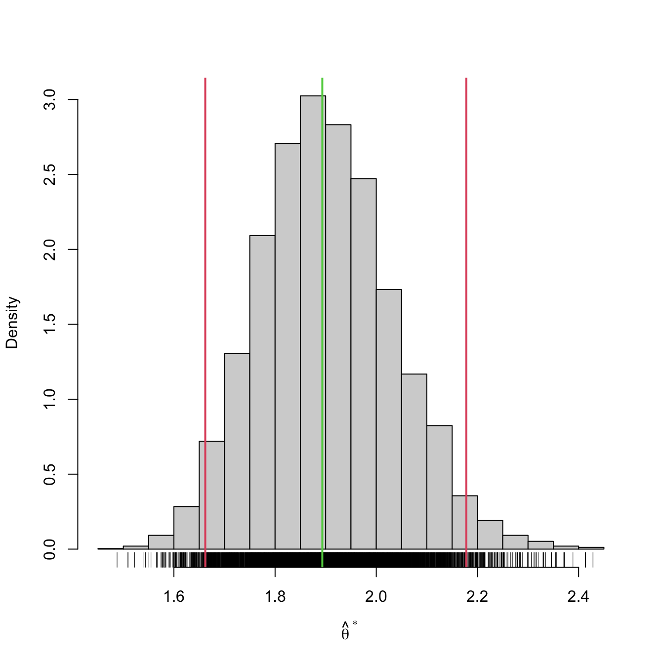
##     2.5%    97.5%
## 1.662018 2.178031
We can compare this confidence interval with that given asymptotically in Example 5.11:
# Asymptotic confidence interval
alpha <- 0.05
z <- qnorm(alpha / 2, lower.tail = FALSE)
lambda_mle <- 1 / mean(x)
lambda_mle + c(-1, 1) * z * lambda_mle / sqrt(n)
## [1] 1.630952 2.155753
Observe the similarity between \(\widehat{\mathrm{CI}}^*_{1-\alpha}(\lambda)\) and \(\mathrm{ACI}_{1-\alpha}(\lambda).\) The bootstrap version has been obtained without using the maximum likelihood theory. It is therefore more general, as it only needs to evaluate \(\hat{\lambda}\) many times. For that reason, it is also much slower to compute than the asymptotic confidence interval, which in turn requires knowing or being able to compute \(\mathcal{I}(\lambda).\)
Example 5.13 The bootstrap confidence interval for the gunpowder data in Example 5.2 is also very similar to the normal confidence interval for the mean obtained there:
# Sample
X <- c(916, 892, 895, 904, 913, 916, 895, 885)

# Bootstrap confidence interval
boot_ci(x = X, B = 5e3, theta_hat = mean)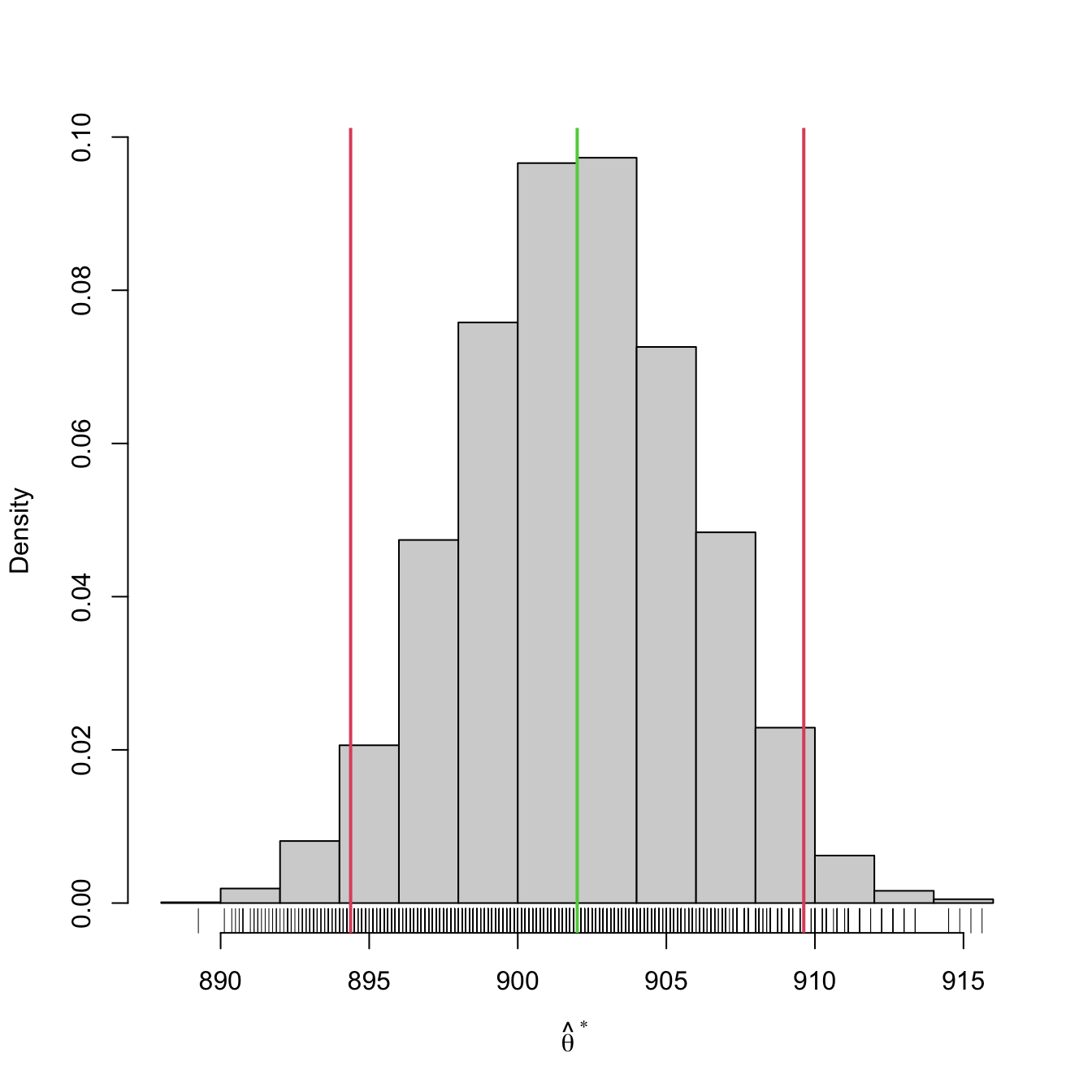
##    2.5%   97.5%
## 894.375 909.625
This step can be excluded if only the confidence interval for \(\hat{\theta}\) is desired, as \(\mathrm{CI}^*_{1-\alpha}(\theta)\) does not depend on \(\hat{\theta}(x_1,\ldots,x_n)\) directly! Nevertheless, it is often useful to know \(\hat{\theta}(x_1,\ldots,x_n)\) in addition to the confidence interval.↩︎
What we do in this step is a Monte Carlo simulation of \(\hat{\theta}^*\) to approximate the sampling distribution of \(\hat{\theta}^*\) with the sample \((\hat{\theta}_1^*,\ldots,\hat{\theta}_B^*).\) In that way, we can approximate \(\mathrm{CI}^*_{1-\alpha}(\theta)\) up to arbitrary precision for a large \(B.\) This precision is quantified through the standard deviation of the Monte Carlo estimate, which is \(C/\sqrt{B}\) with \(C>0\) a fixed constant depending on the problem.↩︎
Replacement, i.e., allowing repetitions of elements in \((X_{1,b}^*,\ldots,X_{n,b}^*),\) is key to generate variability.↩︎
Extracting a sample with replacement from another sample is easy in R: if
xis the vector containing \((x_1,\ldots,x_n),\) thensample(x, replace = TRUE)draws a sample \((X_{1,b}^*,\ldots,X_{n,b}^*).\)↩︎