5.2 Confidence intervals on a normal population

We assume in this section the rv $X$ follows a $\mathcal{N}(\mu,\sigma^2)$ distribution from which a srs $(X_1,\ldots,X_n)$ is extracted. The confidence intervals derived in this section arise from the sampling distributions obtained in Section 2.2 for normal populations. We will apply the pivotal quantity method repeatedly to these sampling distributions.

5.2.1 Confidence interval for the mean with known variance

Let us fix the significance level $\alpha.$ For applying the pivotal quantity method we need an estimator of $\mu$ with known distribution. For example, $\hat{\mu}=\bar{X},$ which verifies

\[\begin{align*} \bar{X}\sim\mathcal{N}\left(\mu,\frac{\sigma^2}{n}\right). \end{align*}\]

A transformation that removes $\mu$ from the distribution of $\bar{X}$ is simply

\[\begin{align*} \bar{X}-\mu\sim\mathcal{N}\left(0,\frac{\sigma^2}{n}\right). \end{align*}\]

However, a more practical pivot is

\[\begin{align} Z:=\frac{\bar{X}-\mu}{\sigma/\sqrt{n}}\sim\mathcal{N}(0,1) \tag{5.3} \end{align}\]

since its distribution is “clean” and does not depend on $\sigma.$

Now we must find the constants $c_1$ and $c_2$ such that

\[\begin{align*} \mathbb{P}(c_1\leq Z\leq c_2)=1-\alpha. \end{align*}\]

If split evenly the probability $\alpha$ at both sides of the distribution,⁶⁵ then $c_1$ and $c_2$ are the constants that verify

\[\begin{align} \Phi(c_1)=\alpha/2\quad \text{and} \quad \Phi(c_2)=1-\alpha/2, \tag{5.4} \end{align}\]

that is, $c_1$ is the lower $\alpha/2$-quantile of $\mathcal{N}(0,1)$ and $c_2$ is the lower $(1-\alpha/2)$-quantile of the same distribution. $c_1$ and $c_2$ are known as critical values.

Definition 5.3 (Critical value) A critical value $\alpha$ of a continuous⁶⁶ rv $X$ is the value of the variable that accumulates $\alpha$ probability to its right, or in other words, is the upper $\alpha$-quantile of $X.$ It is denoted by $x_{\alpha}$ and is such that

\[\begin{align*} \mathbb{P}(X\geq x_{\alpha})=\alpha. \end{align*}\]

The constants $c_1$ and $c_2$ verify

\[\begin{align*} \mathbb{P}(Z\geq c_1)=1-\alpha/2\quad \text{and} \quad \mathbb{P}(Z\geq c_2)=\alpha/2, \end{align*}\]

that is, $c_1=z_{1-\alpha/2}$ and $c_2=z_{\alpha/2}.$ Given the symmetry of the standard normal distribution with respect to $0,$ it is verified that $z_{1-\alpha/2}=-z_{\alpha/2},$ that is, $c_1=-c_2.$ Example 2.8 illustrated how to compute the critical values of a $\mathcal{N}(0,1)$ in R. In terms of the cdf $\Phi$ of $\mathcal{N}(0,1),$ and connecting with (5.4), we have

\[\begin{align*} \Phi(z_{1-\alpha/2})=\Phi(-z_{\alpha/2})=\alpha/2\quad \text{and} \quad \Phi(z_{\alpha/2})=1-\alpha/2. \end{align*}\]

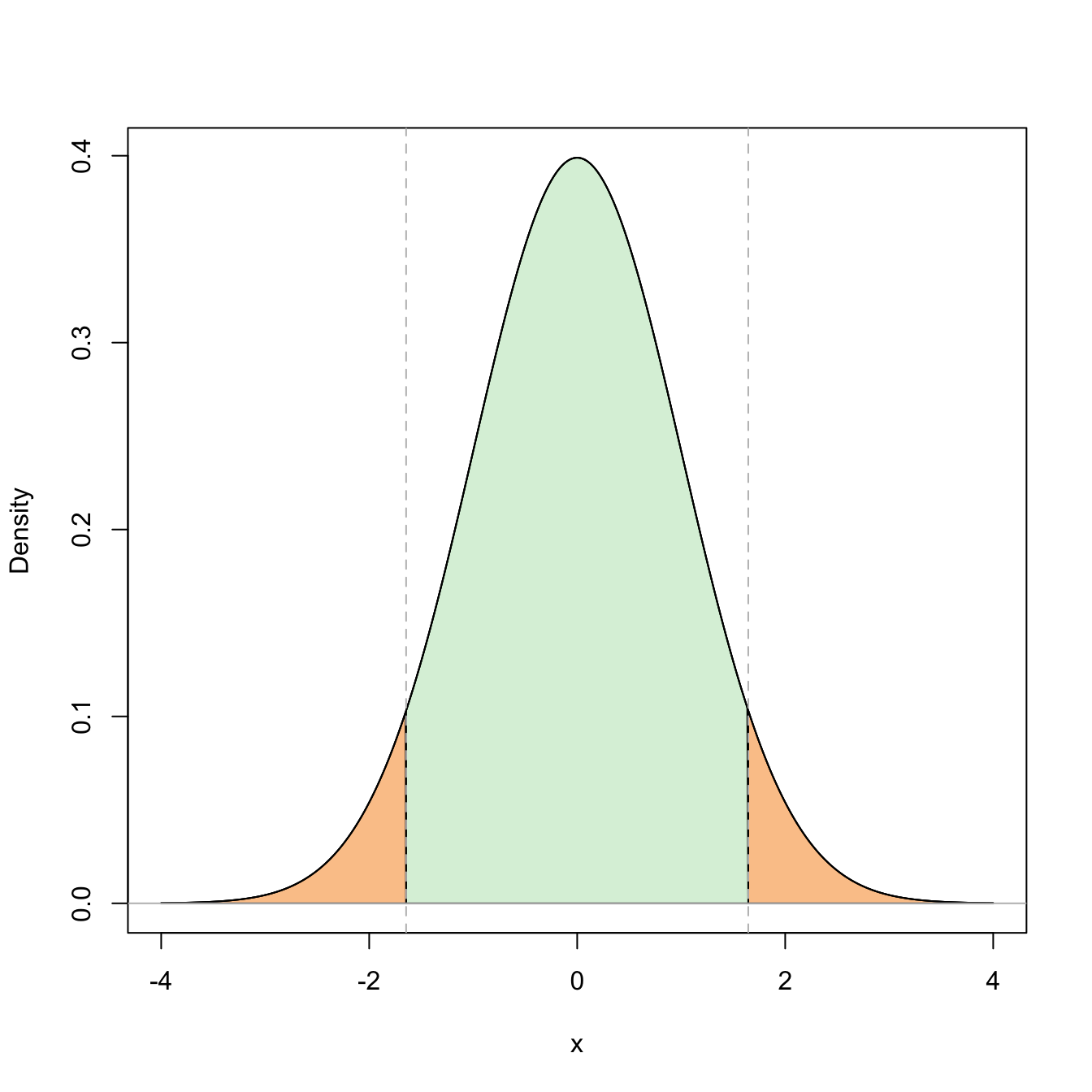
$Representation of the probability $\mathbb{P}(-z_{\alpha/2}\leq Z\leq z_{\alpha/2})=1-\alpha$ (in green) and its complementary (in orange) for $\alpha=0.10$.$

Figure 5.3: Representation of the probability $\mathbb{P}(-z_{\alpha/2}\leq Z\leq z_{\alpha/2})=1-\alpha$ (in green) and its complementary (in orange) for $\alpha=0.10$.

Once obtained $c_1=-z_{\alpha/2}$ and $c_2=z_{\alpha/2},$ we solve for $\mu$ in the inequalities inside the probability:

\[\begin{align*} 1-\alpha &=\mathbb{P}\left(-z_{\alpha/2}\leq \frac{\bar{X}-\mu}{\sigma/\sqrt{n}}\leq z_{\alpha/2}\right)\\ &=\mathbb{P}\left(-z_{\alpha/2}\frac{\sigma}{\sqrt{n}}\leq \bar{X}-\mu\leq z_{\alpha/2}\frac{\sigma}{\sqrt{n}}\right)\\ &=\mathbb{P}\left(-\bar{X}-z_{\alpha/2}\frac{\sigma}{\sqrt{n}}\leq -\mu\leq -\bar{X}+z_{\alpha/2}\frac{\sigma}{\sqrt{n}}\right) \\ &=\mathbb{P}\left(\bar{X}-z_{\alpha/2}\frac{\sigma}{\sqrt{n}}\leq \mu\leq \bar{X}+z_{\alpha/2}\frac{\sigma}{\sqrt{n}}\right). \end{align*}\]

Therefore, a confidence interval for $\mu$ is

\[\begin{align*} \mathrm{CI}_{1-\alpha}(\mu)=\left[\bar{X}-z_{\alpha/2}\frac{\sigma}{\sqrt{n}}, \bar{X}+z_{\alpha/2}\frac{\sigma}{\sqrt{n}}\right]. \end{align*}\]

We represent it in a compact way as

\[\begin{align*} \mathrm{CI}_{1-\alpha}(\mu)=\left[\bar{X}\mp z_{\alpha/2}\frac{\sigma}{\sqrt{n}}\right]. \end{align*}\]

Example 5.2 A gunpowder manufacturer developed a new formula that was tested in eight bullets. The resultant initial velocities, measured in meters per second, were

\[\begin{align*} 916, 892, 895, 904, 913, 916, 895, 885. \end{align*}\]

Assuming that the initial velocities have normal distribution with $\sigma=12$ meters per second, find a confidence interval at significance level $\alpha=0.05$ for the initial mean velocity of the bullets that employ the new gunpowder.

We know that

\[\begin{align*} X\sim \mathcal{N}(\mu,12^2), \ \text{with unknown $\mu$}. \end{align*}\]

From the sample we have that

\[\begin{align*} n=8,\quad \bar{X}=902,\quad \alpha/2=0.025, \quad z_{\alpha/2}\approx1.96. \end{align*}\]

Then, a confidence interval for $\mu$ at $0.95$ confidence is

\[\begin{align*} \mathrm{CI}_{0.95}(\mu)=\left[\bar{X}\mp z_{\alpha/2}\frac{\sigma}{\sqrt{n}}\right]=\left[902\mp z_{\alpha/2}\frac{12}{\sqrt{8}}\right]\approx[893.68, 910.32]. \end{align*}\]

In R, the previous computations can be simply done as:

# Sample
X <- c(916, 892, 895, 904, 913, 916, 895, 885)

# n, mean, sigma, alpha, z_{\alpha/2}
n <- length(X)
X_bar <- mean(X)
sigma <- 12
alpha <- 0.05
z <- qnorm(alpha / 2, lower.tail = FALSE)

# CI
X_bar + c(-1, 1) * z * sigma / sqrt(n)
## [1] 893.6846 910.3154

5.2.2 Confidence interval for the mean with unknown variance

In this case (5.3) is not a pivot: besides depending on $\mu,$ the statistic also depends on another unknown parameter, $\sigma^2,$ which makes impossible to encapsulate $\mu$ between two computable limits. However, we can estimate $\sigma^2$ unbiasedly with $S'^2,$ and produce

\[\begin{align*} T:=\frac{\bar{X}-\mu}{S'/\sqrt{n}}. \end{align*}\]

$T$ is a pivot, since Theorem 2.3 provides the $\mu$-free distribution of $T,$ $t_{n-1}.$ If we split evenly the significance level $\alpha$ between the two tails of the distribution, then the constants $c_1$ and $c_2$ are

\[\begin{align*} \mathbb{P}(c_1\leq T\leq c_2)=1-\alpha, \end{align*}\]

corresponding to the critical values $c_1=t_{n-1;1-\alpha/2}$ and $c_2=t_{n-1;\alpha/2}.$ Since Student’s $t$ is also symmetric, then $c_1=-c_2=-t_{n-1;\alpha/2},$ hence

\[\begin{align*} 1-\alpha=\mathbb{P}\left(-t_{n-1;\alpha/2}\leq \frac{\bar{X}-\mu}{S'/\sqrt{n}}\leq t_{n-1;\alpha/2}\right). \end{align*}\]

Example 2.11 illustrated how to compute probabilities in a Students’$t$ distribution.

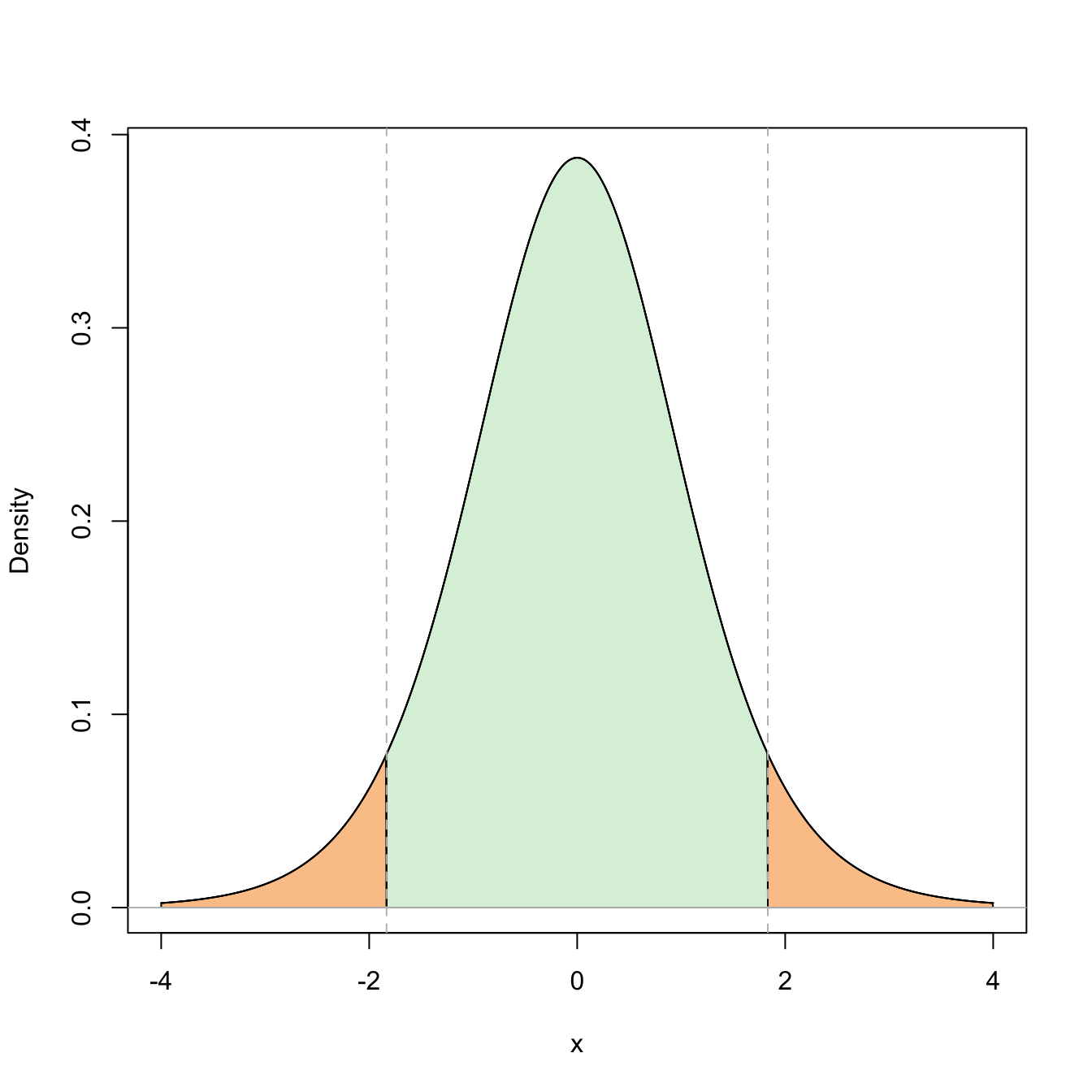
$Representation of the probability $\mathbb{P}(-t_{n-1;\alpha/2}\leq t_{n-1}\leq t_{n-1;\alpha/2})=1-\alpha$ (in green) and its complementary (in orange) for $\alpha=0.10$ and $n=10$.$

Figure 5.4: Representation of the probability $\mathbb{P}(-t_{n-1;\alpha/2}\leq t_{n-1}\leq t_{n-1;\alpha/2})=1-\alpha$ (in green) and its complementary (in orange) for $\alpha=0.10$ and $n=10$.

Solving $\mu$ in the inequalities, we get

\[\begin{align*} 1-\alpha=\mathbb{P}\left(\bar{X}-t_{n-1;\alpha/2}{S'/\sqrt{n}}\leq\mu\leq \bar{X}+t_{n-1;\alpha/2}{S'/\sqrt{n}}\right). \end{align*}\]

Then, a confidence interval for the mean $\mu$ at confidence level $1-\alpha$ is

\[\begin{align*} \mathrm{CI}_{1-\alpha}(\mu)=\left[\bar{X}\mp t_{n-1;\alpha/2}\frac{S'}{\sqrt{n}}\right]. \end{align*}\]

Example 5.3 Compute the same confidence interval asked in the Example 5.2 but assuming that the variance of the initial velocities is unknown.

If the variance is unknown, then we can estimate it with $S'^2=143.43.$ Using $t_{7;0.025}\approx 2.365,$ the confidence interval for $\mu$ is

\[\begin{align*} \mathrm{CI}_{0.95}(\mu)=\left[\bar{X}\mp t_{7;0.025}\frac{S'}{\sqrt{n}}\right]\approx\left[902\mp 2.365\times\sqrt{\frac{143.43}{8}}\right]\approx[891.99, 912.01]. \end{align*}\]

In R, the previous computations can be simply done as:

# Sample
X <- c(916, 892, 895, 904, 913, 916, 895, 885)

# n, mean, S', alpha, t_{\alpha/2;n-1}
n <- length(X)
X_bar <- mean(X)
S_prime <- sd(X)
alpha <- 0.05
t <- qt(alpha / 2, df = n - 1, lower.tail = FALSE)

# CI
X_bar + c(-1, 1) * t * S_prime / sqrt(n)
## [1] 891.9877 912.0123

5.2.3 Confidence interval for the variance

We already have an unbiased estimator of $\sigma^2,$ the quasivariance $S'^2.$ In addition, by Theorem 2.2 we have a pivot

\[\begin{align*} U:=\frac{(n-1)S'^2}{\sigma^2}\sim \chi_{n-1}^2. \end{align*}\]

Then, we only need to compute the constants $c_1$ and $c_2$ such that

\[\begin{align*} \mathbb{P}(c_1\leq U\leq c_2)=1-\alpha. \end{align*}\]

Splitting the probability $\alpha$ evenly to both sides of the $\chi^2$ distribution,⁶⁷ we have that $c_1=\chi_{n-1;1-\alpha/2}^2$ and $c_2=\chi_{n-1;\alpha/2}^2.$ Once the constants are computed, solving for $\sigma^2$ in the inequalities

\[\begin{align*} 1-\alpha &=\mathbb{P}\left(\chi_{n-1;1-\alpha/2}^2\leq \frac{(n-1)S'^2}{\sigma^2} \leq \chi_{n-1;\alpha/2}^2\right)\\ &=\mathbb{P}\left(\frac{\chi_{n-1;1-\alpha/2}^2}{(n-1)S'^2}\leq \frac{1}{\sigma^2} \leq \frac{\chi_{n-1;\alpha/2}^2}{(n-1)S'^2}\right) \\ &=\mathbb{P}\left(\frac{(n-1)S'^2}{\chi_{n-1;\alpha/2}^2}\leq \sigma^2 \leq \frac{(n-1)S'^2}{\chi_{n-1;1-\alpha/2}^2}\right) \end{align*}\]

yields the confidence interval for $\sigma^2$:

\[\begin{align*} \mathrm{CI}_{1-\alpha}(\sigma^2)=\left[\frac{(n-1)S'^2}{\chi_{n-1;\alpha/2}^2}, \frac{(n-1)S'^2}{\chi_{n-1;1-\alpha/2}^2}\right]. \end{align*}\]

Observe that $\chi_{n-1;1-\alpha/2}^2<\chi_{n-1;\alpha/2}^2$ but in the confidence interval these critical values appear in the denominators in reverse order.

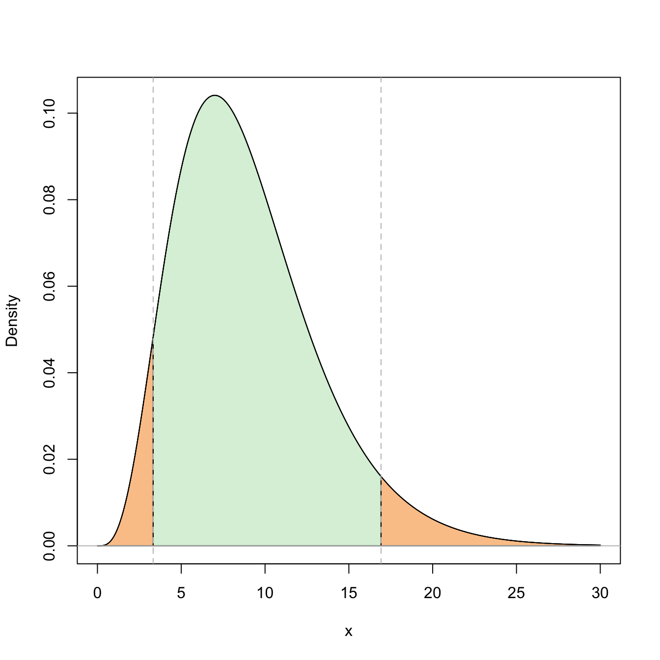
$Representation of the probability $\mathbb{P}(\chi^2_{n-1;1-\alpha/2}\leq \chi^2_{n-1}\leq \chi^2_{n-1;\alpha/2})=1-\alpha$ (in green) and its complementary (in orange) for $\alpha=0.10$ and $n=10$.$

Figure 5.5: Representation of the probability $\mathbb{P}(\chi^2_{n-1;1-\alpha/2}\leq \chi^2_{n-1}\leq \chi^2_{n-1;\alpha/2})=1-\alpha$ (in green) and its complementary (in orange) for $\alpha=0.10$ and $n=10$.

Example 5.4 A practitioner wants to verify the variability of an equipment employed for measuring the volume of an audio source. Three independent measurements recorded with this equipment were

\[\begin{align*} 4.1,\quad 5.2, \quad 10.2. \end{align*}\]

Assuming that the measurements have a normal distribution, obtain the confidence interval of $\sigma^2$ with confidence $0.90.$

From the three measurements we obtain

\[\begin{align*} S'^2=10.57,\quad \alpha/2=0.05,\quad n=3. \end{align*}\]

Then, the confidence interval for $\sigma^2$ is

\[\begin{align*} \mathrm{CI}_{0.90}(\sigma^2)=\left[\frac{(n-1)S'^2}{\chi_{2;0.05}^2},\frac{(n-1)S'^2}{\chi_{2;0.95}^2}\right]\approx\left[\frac{2\times 10.57}{5.991},\frac{2\times 10.57}{0.103}\right]\approx[3.53,205.24]. \end{align*}\]

Recall that since $n$ is small, then the critical value $c_1=\chi_{n;1-\alpha/2}^2$ of the $\chi_{n-1}^2$ distribution is close to zero (see Figure 5.5), and hence the length of the interval is large, illustrating the little information available.

The previous computations can be done as:

# Sample
X <- c(4.1, 5.2, 10.2)

# n, S'^2, alpha, c1, c2
n <- length(X)
S2_prime <- var(X)
alpha <- 0.10
c1 <- qchisq(1 - alpha / 2, df = n - 1, lower.tail = FALSE)
c2 <- qchisq(alpha / 2, df = n - 1, lower.tail = FALSE)

# CI
(n - 1) * S2_prime / c(c2, c1)
## [1]   3.528353 206.069821

This makes a lot of sense in normal distributions due to the shape of the $\mathcal{N}(0,1)$ pdf: symmetric and decaying monotonically from $0.$↩︎
The definition for discrete rv’s involve considering the smallest $x_\alpha$ such that $\mathbb{P}(X\geq x_{\alpha})\geq\alpha.$↩︎
This is due to tradition and simplicity. Unlike in the normal or Student’s $t$ cases, splitting $\alpha$ evenly at both tails does not give the shortest interval containing $1-\alpha$ probability. However, the shortest confidence interval with $1-\alpha$ coverage is more convoluted.↩︎