3.6 Efficient estimators

Definition 3.12 (Fisher information) Let $X\sim f(\cdot;\theta)$ be a continuous rv with $\theta\in\Theta\subset\mathbb{R},$ and such that $\theta\mapsto f(x;\theta)$ is differentiable for all $\theta\in\Theta$ and $x\in \mathrm{supp}(f):=\{x\in\mathbb{R}:f(x;\theta)>0\}$ ($\mathrm{supp}(f)$ is the support of the pdf). The Fisher information of $X$ about $\theta$ is defined as

$$\begin{align} \mathcal{I}(\theta):=\mathbb{E}\left[\left(\frac{\partial \log f(X;\theta)}{\partial \theta}\right)^2\right].\tag{3.7} \end{align}$$

When $X$ is discrete, the Fisher information is defined analogously by just replacing the pdf $f(\cdot;\theta)$ by the pmf $p(\cdot;\theta).$

Observe that the quantity

$$\begin{align} \left(\frac{\partial \log f(x;\theta)}{\partial \theta}\right)^2=\left(\frac{1}{f(x;\theta)}\frac{\partial f(x;\theta)}{\partial \theta}\right)^2 \tag{3.8} \end{align}$$

is the square of the weighted rate of variation of $\theta\mapsto f(x;\theta)$ for infinitesimal variations of $\theta,$ for the realization $x$ of the rv $X.$ The square is meant to remove the sign from the rate of variation. Therefore, (3.8) can be interpreted as the information contained in $x$ for discriminating the parameter $\theta$ from close values $\theta+\delta.$ For example, if (3.8) is close to zero for $\theta=\theta_0,$ then it means that $\theta\mapsto f(x;\theta)$ is almost flat about $\theta=\theta_0,$ so $f(x;\theta_0)$ and $f(x;\theta_0+\delta)$ are very similar. This means that the sample realization $X=x$ is not informative on whether the underlying parameter $\theta$ is $\theta_0$ or $\theta_0+\delta$ because both have almost the same likelihood.

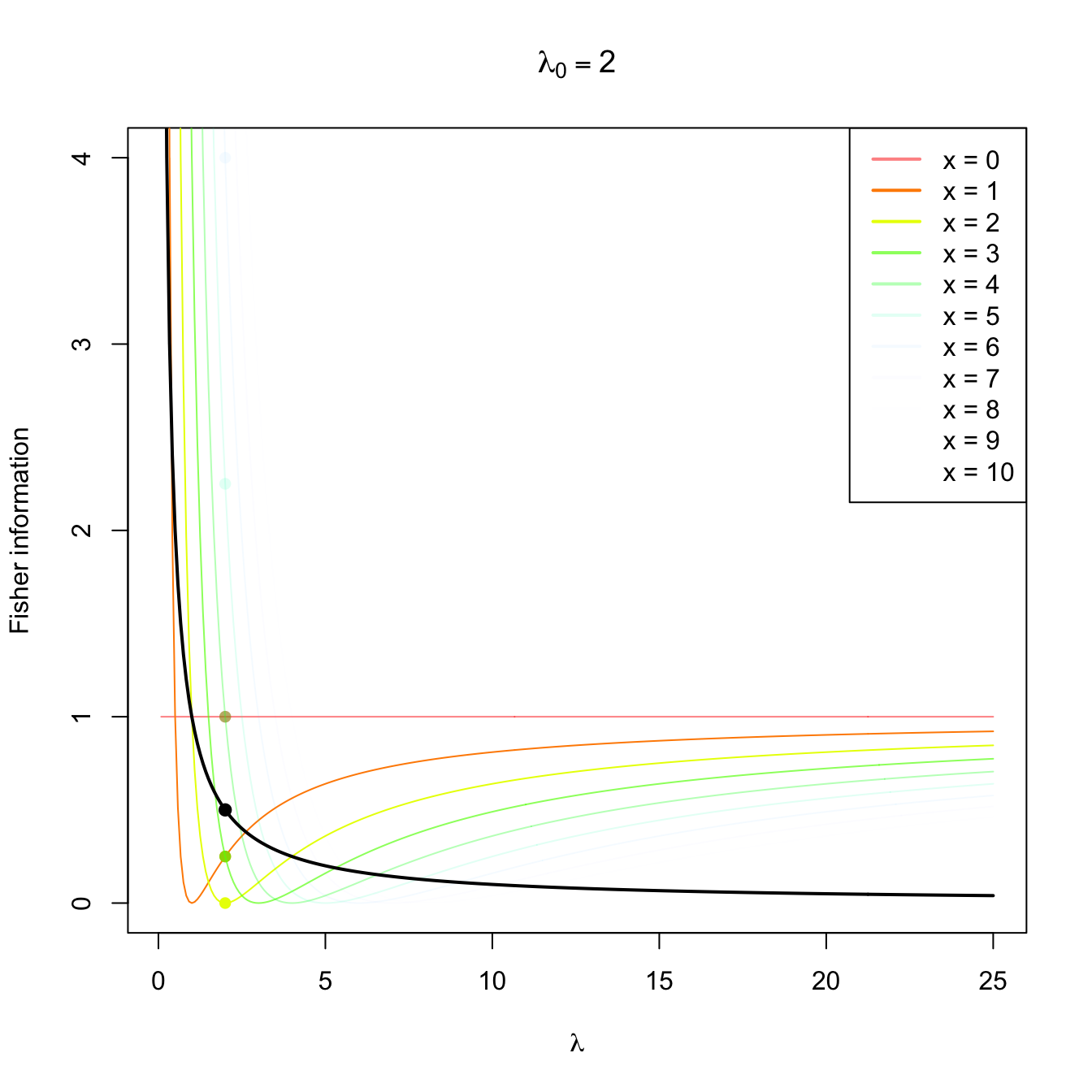
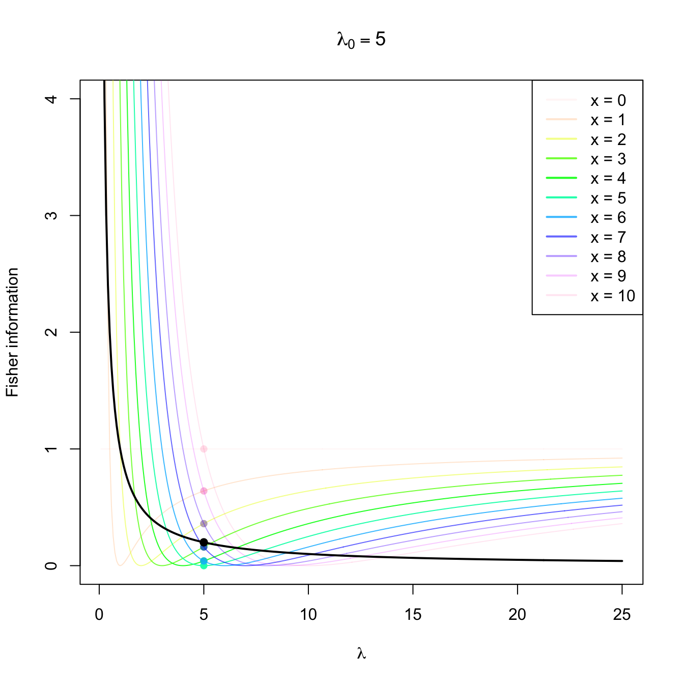
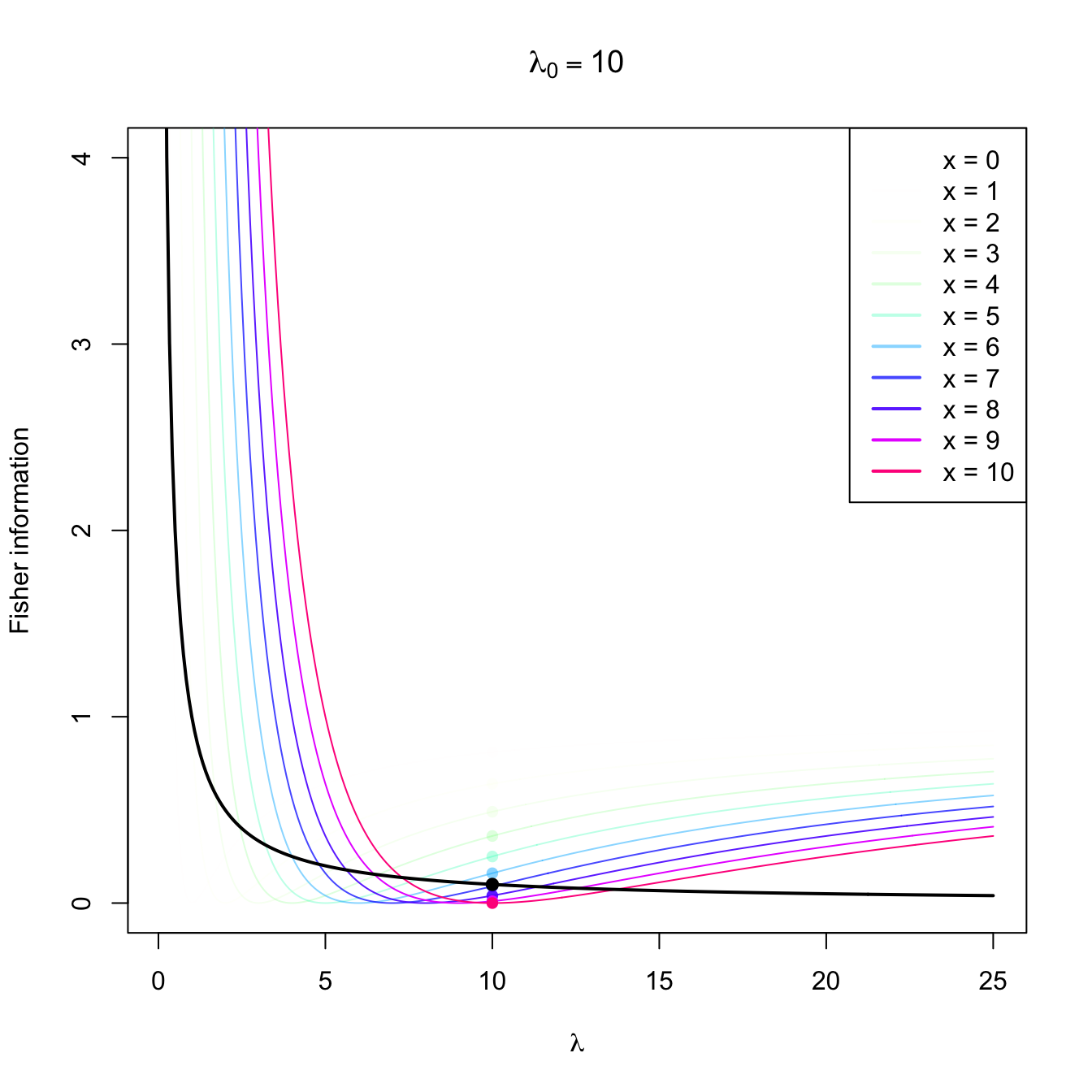
Figure 3.4: Fisher information integrand $\lambda\mapsto \left(\partial \log f(x;\lambda)/\partial \lambda\right)^2$ in a $\mathrm{Pois}(\lambda_0)$ distribution with $\lambda_0=2,5,10.$ The integrands are shown in different colors, with the color transparency indicating the probability of $x$ according to $\mathrm{Pois}(\lambda_0)$ (the darker the color, the higher the probability). The Fisher information curve $\lambda\mapsto \mathcal{I}(\lambda)$ is shown in black, with a black point signaling the value $\mathcal{I}(\lambda_0).$ The colored points indicate the contribution of each $x$ to the Fisher information.

When taking the expectation in (3.7), we obtain that the Fisher information is the expected information of $X$ that is useful to distinguish $\theta$ from close values. This quantity is related with the precision (i.e., the inverse of the variance) of an unbiased estimator of $\theta.$

Example 3.30 Compute the Fisher’s information of a rv $X\sim \mathrm{Pois}(\lambda).$

The Poisson’s pmf is given by

$$\begin{align*} p(x;\lambda)=\frac{\lambda^x e^{-\lambda}}{x!}, \quad x=0,1,2,\ldots, \end{align*}$$

so its logarithm is

$$\begin{align*} \log{p(x;\lambda)}=x\log{\lambda}-\lambda-\log{(x!)} \end{align*}$$

and its derivative with respect to $\lambda$ is

$$\begin{align*} \frac{\partial \log p(x;\lambda)}{\partial \lambda}=\frac{x}{\lambda}-1. \end{align*}$$

The Fisher information is then obtained taking the expectation of³⁹

$$\begin{align*} \left(\frac{\partial \log p(X;\lambda)}{\partial \lambda}\right)^2=\left(\frac{X-\lambda}{\lambda}\right)^2, \end{align*}$$

Noting that $\mathbb{E}[X]=\lambda$ and, therefore, $\mathbb{E}[(X-\lambda)^2]=\mathbb{V}\mathrm{ar}[X]=\lambda,$ we obtain

$$\begin{align} \mathcal{I}(\lambda)=\mathbb{E}\left[\left(\frac{X-\lambda}{\lambda}\right)^2\right]=\frac{\mathbb{V}\mathrm{ar}[X]}{\lambda^2}=\frac{1}{\lambda}.\tag{3.9} \end{align}$$

The following fundamental result states the lower variance bound of an unbiased estimator that is regular enough. Hence, it establishes the lowest MSE that an unbiased estimator can attain and thus establishes a reference for other unbiased estimators. The inequality is also known as the information inequality.

Theorem 3.8 (Crámer–Rao’s inequality) Let $(X_1,\ldots,X_n)$ be a srs of a rv with pdf $f(x;\theta),$ and let $$\begin{align*} \mathcal{I}_n(\theta):=n\mathcal{I}(\theta) \end{align*}$$ be the Fisher’s information of the sample $(X_1,\ldots,X_n)$ about $\theta.$ If $\hat{\theta}\equiv\hat{\theta}(X_1,\ldots,X_n)$ is an unbiased estimator of $\theta$ then, under certain general conditions,⁴⁰ it holds

$$\begin{align*} \mathbb{V}\mathrm{ar}\big[\hat{\theta}\big]\geq \frac{1}{\mathcal{I}_n(\theta)}. \end{align*}$$

Definition 3.13 (Efficient estimator) An unbiased estimator $\hat{\theta}$ of $\theta$ that verifies $\mathbb{V}\mathrm{ar}\big[\hat{\theta}\big]=(\mathcal{I}_n(\theta))^{-1}$ is said to be efficient.

Example 3.31 Show that for a rv $\mathrm{Pois}(\lambda)$ the estimator $\hat{\lambda}=\bar{X}$ is efficient.

We first calculate the Fisher information $\mathcal{I}_n(\theta)$ of the sample $(X_1,\ldots,X_n).$ Since $\mathcal{I}(\lambda)=1/\lambda$ from Example 3.30, then

$$\begin{align*} \mathcal{I}_n(\lambda)&=n\mathcal{I}(\lambda)=\frac{n}{\lambda}. \end{align*}$$

On the other hand, the variance of $\hat{\lambda}=\bar{X}$ is

$$\begin{align*} \mathbb{V}\mathrm{ar}[\hat{\lambda}]=\frac{1}{n^2}\mathbb{V}\mathrm{ar}\left[\sum_{i=1}^n X_i\right]=\frac{n\lambda}{n^2}=\frac{\lambda}{n}. \end{align*}$$

Therefore, $\hat{\lambda}=\bar{X}$ is efficient.

Example 3.32 Check that $\hat{\theta}=\bar{X}$ is efficient for estimating $\theta$ in a population $\mathrm{Exp}(1/\theta).$

References

Lehmann, E. L., and G. Casella. 1998. Theory of Point Estimation. Second. Springer Texts in Statistics. New York: Springer-Verlag. https://doi.org/10.1007/b98854.

---

39. Note that we change $x$ to $X$ because now we have to work with a random variable to take an expectation.↩︎

40. See Theorem 5.10 (Section 2.5, page 120) in Lehmann and Casella (1998).↩︎