1.3 Random vectors

A random vector is just a collection of random variables generated by the same measurable space $(\Omega,\mathcal{A})$ associated to an experiment $\xi.$ Before formally defining them, we need to generalize Definition 1.4.

Definition 1.22 (Borel $\sigma$-algebra in $\mathbb{R}^p$) Let $\Omega=\mathbb{R}^p,$ $p\geq 1.$ Consider the collection of hyperrectangles

\[\begin{align*} \mathcal{I}^p:=\{(-\infty,a_1]\times\stackrel{p}{\cdots} \times(-\infty,a_p]: a_1,\ldots,a_p\in \mathbb{R}\}. \end{align*}\]

The Borel $\sigma$-algebra in $\mathbb{R^p}$, denoted by $\mathcal{B}^p,$ is defined as the smallest $\sigma$-algebra that contains $\mathcal{I}^p.$

Definition 1.23 (Random vector) Let $(\Omega,\mathcal{A})$ be measurable space. Let $\mathcal{B}^p$ be the Borel $\sigma$-algebra over $\mathbb{R}^p.$ A random vector is a mapping $\boldsymbol{X}:\Omega\rightarrow \mathbb{R}^p$ that is measurable, that is, that verifies

\[\begin{align*} \forall B\in\mathcal{B}^p, \quad \boldsymbol{X}^{-1}(B)\in\mathcal{A}, \end{align*}\]

with $\boldsymbol{X}^{-1}(B)=\{\omega\in\Omega: \boldsymbol{X}(\omega)\in B\}.$

It is clear that the above generalizes Definition 1.13, which follows for $p=1.$ It is nevertheless simpler to think about random vectors in terms of the following characterization, which states that a random vector is indeed just a collection of random variables.

Proposition 1.6 Given a measurable space $(\Omega,\mathcal{A}),$ a mapping $\boldsymbol{X}:\Omega\rightarrow \mathbb{R}^p$ defined as $\boldsymbol{X}(\omega)=(X_1(\omega),\ldots,X_p(\omega))'$ is a random vector if and only if $X_1,\ldots,X_p:\Omega\rightarrow \mathbb{R}$ are random variables in $(\Omega,\mathcal{A}).$¹⁴

Example 1.24 Let $\xi=$ “Roll a dice $10$ times”. Then, $\#\Omega=6^{10}.$ We can define the random vector $\boldsymbol{X}(\omega)=(X_1(\omega),X_2(\omega))'$ where $X_1(\omega)=$ “Number of $5$’s in $\omega$” and $X_2(\omega)=$ “Number of $3$’s in $\omega$” ($\omega$ is the random output of $\xi,$ i.e., the information of the obtained $10$ sides of the rolled dice).

It can be seen that $\boldsymbol{X}$ is a random vector, comprised by the random variables $X_1$ and $X_2,$ with respect to the measurable space $(\Omega,\mathcal{P}(\Omega)).$

As a random variable does, a random vector $\boldsymbol{X}$ also induces a probability $\mathbb{P}_{\boldsymbol{X}}$ over $(\mathbb{R}^p,\mathcal{B}^p)$ from a probability $\mathbb{P}$ in $(\Omega,\mathcal{A}).$ The following is an immediate generalization of Definition 1.14.

Definition 1.24 (Induced probability of a random vector) Let $\mathcal{B}^p$ be the Borel $\sigma$-algebra over $\mathbb{R}^p.$ The induced probability of the random vector $\boldsymbol{X}$ is the function $\mathbb{P}_{\boldsymbol{X}}:\mathcal{B}^p\rightarrow \mathbb{R}^p$ defined as

\[\begin{align*} \mathbb{P}_{\boldsymbol{X}}(B):=\mathbb{P}(\boldsymbol{X}^{-1}(B)), \quad \forall B\in \mathcal{B}^p. \end{align*}\]

Example 1.25 In Example 1.24, a probability for $\xi$ that is compatible with common belief is $\mathbb{P}(\{\omega\})=6^{-10},$ $\forall\omega\in\Omega.$ With this probability, we have a probability space $(\Omega,\mathcal{A},\mathbb{P}).$ The induced probability $\mathbb{P}_{\boldsymbol{X}}$ could be worked out from this probability.

In the previous example, the induced probability by $\boldsymbol{X}$ can be computed following Definition 1.24, thus generating the probability space $(\mathbb{R}^2,\mathcal{B}^2,\mathbb{P}_{\boldsymbol{X}}).$ However, as indicated with random variables, we will not need to do this in practice: we will directly specify $\mathbb{P}_{\boldsymbol{X}}$ via probability models, in this case for random vectors, and forget about the conceptual pillars on which $\mathbb{P}_{\boldsymbol{X}}$ is built (the random experiment $\xi$ and the probability space $(\Omega,\mathcal{A},\mathbb{P})$). Again, for introducing probability models, we need to distinguish first among the two most common types of random vectors: discrete and continuous.

1.3.1 Types of random vectors

Definition 1.25 (Joint cdf for random vectors) The joint cumulative distribution function (joint cdf or simply cdf) of a random vector $\boldsymbol{X}$ is the function $F_{\boldsymbol{X}}:\mathbb{R}^p\rightarrow [0,1]$ defined as

\[\begin{align*} F_{\boldsymbol{X}}(\boldsymbol{x}):=\mathbb{P}_{\boldsymbol{X}}((-\infty,x_1]\times\stackrel{p}{\cdots}\times(-\infty,x_p]), \quad \forall \boldsymbol{x}=(\boldsymbol{x}_1,\ldots, \boldsymbol{x}_p)'\in \mathbb{R}. \end{align*}\]

We will denote $\mathbb{P}(\boldsymbol{X}\leq \boldsymbol{x}):=\mathbb{P}_{\boldsymbol{X}}((-\infty,x_1]\times\stackrel{p}{\cdots}\times(-\infty,x_p])$ for simplicity.

Remark. The notation $\mathbb{P}(\boldsymbol{X}\leq \boldsymbol{x})$ equivalently means

\[\begin{align*} \mathbb{P}(\boldsymbol{X}\leq \boldsymbol{x})&=\mathbb{P}(X_1\leq x_1,\ldots,X_p\leq x_p)\\ &=\mathbb{P}(\{X_1\leq x_1\}\cap \ldots\cap \{X_p\leq x_p\}). \end{align*}\]

Proposition 1.7 (Properties of the joint cdf)

The cdf is monotonically non-decreasing, in each component, that is, \[\begin{align*} x_i<y_i \implies F_{\boldsymbol{X}}(\boldsymbol{x})\leq F_{\boldsymbol{X}}(\boldsymbol{y}),\quad \text{for any }i=1,\ldots,p. \end{align*}\]
$\lim_{x_i\to-\infty} F(\boldsymbol{x})=0$ for any $i=1,\ldots,p.$
$\lim_{\boldsymbol{x}\to+\boldsymbol{\infty}} F(\boldsymbol{x})=1.$
$F_{\boldsymbol{X}}$ is right-continuous.¹⁵

Definition 1.26 (Discrete random vector) A random vector $\boldsymbol{X}$ is discrete if its range (or image set) $R_{\boldsymbol{X}}:=\{\boldsymbol{x}\in \mathbb{R}^p: \boldsymbol{x}=\boldsymbol{X}(\omega)\ \text{for some} \ \omega\in \Omega\}$ is finite or countable.

Definition 1.27 (Joint pmf for random vectors) The probability mass function (pmf) of a discrete random vector $\boldsymbol{X}$ is the function $p_{\boldsymbol{X}}:\mathbb{R}^p\rightarrow [0,1]$ such

\[\begin{align*} p_{\boldsymbol{X}}(\boldsymbol{x}):=\mathbb{P}_{\boldsymbol{X}}(\{\boldsymbol{x}\}), \quad \forall \boldsymbol{x}\in \mathbb{R}^p. \end{align*}\]

The notation $\mathbb{P}(\boldsymbol{X}=\boldsymbol{x}):=p_{\boldsymbol{X}}(\boldsymbol{x})$ is also often employed.

Definition 1.28 (Continuous random vector) A continuous random vector $\boldsymbol{X}$ (also denoted absolutely continuous) is the one whose cdf $F_{\boldsymbol{X}}$ is expressible as

\[\begin{align*} F_{\boldsymbol{X}}(\boldsymbol{x})&=\int_{-\infty}^{x_1}\cdots\int_{-\infty}^{x_p} f_{\boldsymbol{X}}(t_1,\ldots,t_p)\,\mathrm{d}t_p\cdots\mathrm{d}t_1,\quad\forall \boldsymbol{x}\in\mathbb{R}^p, \end{align*}\]

where $f_{\boldsymbol{X}}:\mathbb{R}^p\rightarrow[0,\infty).$ The function $f_{\boldsymbol{X}}$ is the joint probability density function (joint pdf or simply pdf) of $\boldsymbol{X}.$

Proposition 1.8 (Properties of the joint pdf)

$\frac{\partial^p}{\partial x_1\cdots\partial x_p}F_{\boldsymbol{X}}(\boldsymbol{x})=f_{\boldsymbol{X}}(\boldsymbol{x})$ for almost all $\boldsymbol{x}\in\mathbb{R}^p.$¹⁶
$f$ is non-negative and such that \[\begin{align*} \int_{-\infty}^{\infty}\cdots\int_{-\infty}^{\infty} f_{\boldsymbol{X}}(t_1,\ldots,t_p)\,\mathrm{d}t_p\cdots\mathrm{d}t_1=\int_{\mathbb{R}^p} f_{\boldsymbol{X}}(\boldsymbol{t})\,\mathrm{d}\boldsymbol{t}=1. \end{align*}\]
For $A\in\mathcal{B}^p,$ $\mathbb{P}(\boldsymbol{X}\in A)=\int_{A} f_{\boldsymbol{X}}(\boldsymbol{t})\,\mathrm{d}\boldsymbol{t}.$¹⁷

Remark. As for random variables, recall that the cdf accumulates probability irrespective of the type of the random vector. Probability assignment to specific values of $\boldsymbol{X}$ is a type-dependent operation.

Example 1.26 (Uniform random vector) Take $\boldsymbol{X}\sim\mathcal{U}([0,1]\times[0,2]).$ The joint pdf of $\boldsymbol{X}$ is

\[\begin{align*} f(x_1,x_2)=\begin{cases} 1/2,&(x_1,x_2)'\in[0,1]\times[0,2],\\ 0,&\text{otherwise.} \end{cases} \end{align*}\]

The joint cdf of $\boldsymbol{X}$ is

\[\begin{align*} F(x_1,x_2)=\int_{-\infty}^{x_1}\int_{-\infty}^{x_2}f(t_1,t_2)\,\mathrm{d}t_2\,\mathrm{d}t_1. \end{align*}\]

Therefore, carefully taking into account the definition of $f,$ we get

\[\begin{align*} F(x_1,x_2)=\begin{cases} 0,&x_1<0\text{ or }x_2<0,\\ x_1,&0\leq x_1\leq 1,x_2>2,\\ (x_1x_2)/2,&0\leq x_1\leq 1,0\leq x_2\leq 2,\\ x_2/2,&x_1> 1,0\leq x_2\leq 2,\\ 1,&x_1>1,x_2>2. \end{cases} \end{align*}\]

Example 1.27 (A discrete random vector) Let $\boldsymbol{X}=(X_1,X_2)',$ where $X_1\sim\mathcal{U}(\{1,2,3\})$ and $X_2\sim \mathrm{Bin}(1, 2/3)$ (both variables are independent of each other). This means that:

$\mathbb{P}(X_1=x)=1/3,$ for $x=1,2,3$ (and zero otherwise).
$\mathbb{P}(X_2=1)=2/3$ and $\mathbb{P}(X_2=0)=1/3$ (and zero otherwise).
$\mathbb{P}(X_1=x_1,X_2=x_2)=\mathbb{P}(X_1=x_1)\mathbb{P}(X_2=x_2).$
The atoms of $\boldsymbol{X}$ are $\{(1,0),(2,0),(3,0),(1,1),(2,1),(3,1)\}.$

Let us compute the cdf $F$ evaluated at $(5/2,1/2)$:

\[\begin{align*} F(5/2,1/2)&=\mathbb{P}(X_1\leq 5/2,X_2\leq 1/2)\\ &=\mathbb{P}(X_1=1,X_2=0)+\mathbb{P}(X_1=2,X_2=0)\\ &=(1/3)^2 + (1/3)^2\\ &=2/9. \end{align*}\]

1.3.2 Marginal distributions

The joint cdf/pdf/pmf characterize the joint random behavior of $\boldsymbol{X}.$ What about the behavior of each component of $\boldsymbol{X}$?

Definition 1.29 (Marginal cdf) The $i$-th marginal cumulative distribution function (marginal cdf) of a random vector $\boldsymbol{X}$ is defined as

\[\begin{align*} F_{X_i}(x_i):=&\;F_{\boldsymbol{X}}(\infty,\ldots,\infty,x_i,\infty,\ldots,\infty)\\ =&\;\mathbb{P}(X_1\leq \infty,\ldots,X_i\leq x_i,\ldots,X_p\leq \infty)\\ =&\;\mathbb{P}(X_i\leq x_i). \end{align*}\]

Definition 1.30 (Marginal pdf) The $i$-th marginal probability density function (marginal pdf) of a random vector $\boldsymbol{X}$ is defined as

\[\begin{align*} f_{X_i}(x_i):=&\;\frac{\partial}{\partial x_i}F_{X_i}(x_i)\\ =&\;\int_{-\infty}^{\infty}\stackrel{p-1}{\cdots}\int_{-\infty}^{\infty} f_{\boldsymbol{X}}(x_1,\ldots,x_i,\ldots,x_p)\,\mathrm{d}x_p\stackrel{p-1}{\cdots}\mathrm{d}x_1\\ =&\;\int_{\mathbb{R}^{p-1}} f_{\boldsymbol{X}}(\boldsymbol{x})\,\mathrm{d}\boldsymbol{x}_{-i}, \end{align*}\]

where $\boldsymbol{x}_{-i}=(x_1,\ldots,x_{i-1},x_{i+1},\ldots,x_p)'$ is the vector $\boldsymbol{x}$ without the $i$-th entry.

Definition 1.31 (Marginal pmf) The $i$-th marginal probability mass function (marginal pmf) of a random vector $\boldsymbol{X}$ is defined as

\[\begin{align*} p_{X_i}(x_i):=\sum_{\{x_1\in\mathbb{R}:p_{X_1}(x_1)>0\}}\stackrel{p-1}{\cdots}\sum_{\{x_p\in\mathbb{R}:p_{X_p}(x_p)>0\}} p_{\boldsymbol{X}}(x_1,\ldots,x_i,\ldots,x_p). \end{align*}\]

Getting marginal cdfs/pdfs/pmfs from joint cdf/pdf/pmf is always possible. What about the converse?

1.3.3 Conditional distributions

Just as the cdf/pdf/pmf of a random vector allows us to easily work with the probability function $\mathbb{P}$ of a probability space $(\Omega,\mathcal{A},\mathbb{P}),$ the conditional cdf/pdf/pmf of a random variable¹⁸ given another will serve to work with the conditional probability as defined in Definition 1.11. To help out with the intuition of the following definitions, recall that we can re-express (1.1) as

\[\begin{align*} \mathbb{P}(A\textbf{ conditioned to } B):=\frac{\mathbb{P}(\text{$A$ and $B$ } \textbf{jointly})}{\mathbb{P}(B\textbf{ alone})}. \end{align*}\]

Conditional distributions allow answering the next question: if we have a random vector $(X_1,X_2)',$ what can we say about the randomness of $X_2|X_1=x_1$? Conditional distributions are type-dependent; we see them next for continuous and discrete rv’s.

Definition 1.32 (Conditional pdf and cdf for a continuous random vector) Given a continuous random vector $\boldsymbol{X}=(X_1,X_2)'$ with joint pdf $f_{\boldsymbol{X}},$ the conditional pdf of $X_1$ given $X_2=x_2$, $f_{X_2}(x_2)>0,$ is the pdf of the continuous random variable $X_1|X_2=x_2$:

\[\begin{align} f_{X_1|X_2=x_2}(x_1):=\frac{f_{\boldsymbol{X}}(x_1,x_2)}{f_{X_2}(x_2)}.\tag{1.4} \end{align}\]

The conditional cdf of $X_1$ given $X_2=x_2$ is

\[\begin{align*} F_{X_1|X_2=x_2}(x_1)=\int_{-\infty}^{x_1}f_{X_1|X_2=x_2}(t)\mathrm{d}t. \end{align*}\]

Definition 1.33 (Conditional pmf and cdf for a discrete random vector) Given a discrete random vector $\boldsymbol{X}=(X_1,X_2)'$ with joint pmf $p_{\boldsymbol{X}},$ the conditional pmf of $X_1$ given $X_2=x_2$, $p_{X_2}(x_2)>0,$ is the pmf of the discrete random variable $X_1|X_2=x_2$:

\[\begin{align} p_{X_1|X_2=x_2}(x_1):=\frac{p_{\boldsymbol{X}}(x_1,x_2)}{p_{X_2}(x_2)}.\tag{1.5} \end{align}\]

The conditional cdf of $X_1$ given $X_2=x_2$ is

\[\begin{align*} F_{X_1|X_2=x_2}(x_1)=\sum_{\{x\in\mathbb{R}:p_{X_1|X_2=x_2}(x)>0,\,x\leq x_1\}}p_{X_1|X_2=x_2}(x). \end{align*}\]

Remark. Recall the similarities of (1.4) and (1.5) with (1.1).

Remark. Recall that the conditional pdf/pmf/cdf of $X_1$ given $X_2=x_2$ is a family of functions, each with argument $x_1,$ that is indexed by the values $X_2=x_2.$

The conditional cdf/pdf/pmf of $X_2$ given $X_1=x_1$ are defined analogously to Definitions 1.32 and 1.33. The previous definitions can be extended to account for conditioning of one random vector onto another with similar constructions.

Remark. Mixed types of conditioning, such as “discrete|continuous” or “continuous|discrete” are possible, but require the consideration of singular random vectors. These types of random vectors are neither continuous nor discrete, but a mix of them, and are more complex.

Once we have the notion of joint, marginal, and conditional distributions, we are in position of defining when two random variables are independent between them. This will resemble Definition 1.12. Indeed, we can define the concept of independence from different angles, as collected in the following definition.

Definition 1.34 (Independent random variables) Two random variables $X_1$ and $X_2$ are independent if and only if

\[\begin{align*} F_{\boldsymbol{X}}(x_1,x_2)=F_{X_1}(x_1)F_{X_2}(x_2),\quad \forall (x_1,x_2)'\in\mathbb{R}^2, \end{align*}\]

where $\boldsymbol{X} =(X_1,X_2)'.$ Equivalently:

If $\boldsymbol{X}$ is continuous, $X_1$ and $X_2$ are independent if and only if \[\begin{align} f_{\boldsymbol{X}}(x_1,x_2)=f_{X_1}(x_1)f_{X_2}(x_2),\quad \forall (x_1,x_2)'\in\mathbb{R}^2.\tag{1.6} \end{align}\]
If $\boldsymbol{X}$ is discrete, $X_1$ and $X_2$ are independent if and only if \[\begin{align} p_{\boldsymbol{X}}(x_1,x_2)=p_{X_1}(x_1)p_{X_2}(x_2),\quad \forall (x_1,x_2)'\in\mathbb{R}^2.\tag{1.7} \end{align}\]

In virtue of the conditional pdf/pmf, the following are equivalent definitions to (1.6) and (1.7):

If $\boldsymbol{X}$ is continuous, $X_1$ and $X_2$ are independent if and only if \[\begin{align*} f_{X_1|X_2=x_2}(x_1)=f_{X_1}(x_1),\quad \forall (x_1,x_2)'\in\mathbb{R}^2. \end{align*}\]
If $\boldsymbol{X}$ is discrete, $X_1$ and $X_2$ are independent if and only if \[\begin{align*} p_{X_1|X_2=x_2}(x_1)=p_{X_1}(x_1),\quad \forall (x_1,x_2)'\in\mathbb{R}^2. \end{align*}\]

Definition 1.34 is also immediately applicable to collections of $p>2$ random variables. Indeed, the random variables in $\boldsymbol{X}=(X_1,\ldots,X_p)'$ are (mutually) independent if and only if \[\begin{align} F_{\boldsymbol{X}}(\boldsymbol{x})=\prod_{i=1}^pF_{X_i}(x_i),\quad \forall \boldsymbol{x}\in\mathbb{R}^p. \tag{1.8} \end{align}\]

If $\boldsymbol{X}$ is continuous/discrete, then (1.8) is equivalent to the factorization of the joint pdf/pmf into its marginals.

1.3.4 Expectation and variance-covariance matrix

Definition 1.35 (Expectation of a random vector) Given a random vector $\boldsymbol{X}\sim F_{\boldsymbol{X}}$ in $\mathbb{R}^p,$ its expectation $\mathbb{E}[\boldsymbol{X}],$ a vector in $\mathbb{R}^p,$ is defined as

\[\begin{align*} \mathbb{E}[\boldsymbol{X}]:=&\;\int \boldsymbol{x}\,\mathrm{d}F_{\boldsymbol{X}}(\boldsymbol{x})\\ :=&\;\begin{cases} \displaystyle\int_{\mathbb{R}^p} \boldsymbol{x} f_{\boldsymbol{X}}(\boldsymbol{x})\,\mathrm{d}\boldsymbol{X},&\text{ if }\boldsymbol{X}\text{ is continuous,}\\ \displaystyle\sum_{\{\boldsymbol{x}\in\mathbb{R}^p:p_{\boldsymbol{X}}(\boldsymbol{x})>0\}} \boldsymbol{x}p_{\boldsymbol{X}}(\boldsymbol{x}),&\text{ if }\boldsymbol{X}\text{ is discrete.} \end{cases} \end{align*}\]

Recall that the expectation $\mathbb{E}[\boldsymbol{X}]$ is just the vector of marginal expectations $(\mathbb{E}[X_1],\ldots,\mathbb{E}[X_p])'.$ That is, if $\boldsymbol{X}$ is continuous, then

\[\begin{align*} \mathbb{E}[\boldsymbol{X}]=&\;(\mathbb{E}[X_1],\ldots,\mathbb{E}[X_p])'\\ =&\;\left(\int_{\mathbb{R}} x_1 f_{X_1}(x_1)\,\mathrm{d}x_1,\ldots, \int_{\mathbb{R}} x_p f_{X_p}(x_p)\,\mathrm{d}x_p\right)'. \end{align*}\]

Example 1.28 Let $\boldsymbol{X}=(X_1,X_2)'$ be a random vector with joint pdf $f(x,y)=e^{-(x+y)}1_{\{x,y>0\}}$ (check that it integrates one). Then:

\[\begin{align*} \mathbb{E}[\boldsymbol{X}]=&\;\int_{\mathbb{R}^2} (x,y)' f(x,y)\,\mathrm{d}x\,\mathrm{d}y\\ =&\;\left(\int_{\mathbb{R}^2} x f(x,y)\,\mathrm{d}x\,\mathrm{d}y,\int_{\mathbb{R}^2} y f(x,y)\,\mathrm{d}x\,\mathrm{d}y\right)'\\ =&\;\left(\int_{0}^\infty\int_{0}^\infty x e^{-(x+y)}\,\mathrm{d}x\,\mathrm{d}y,\int_{0}^\infty\int_{0}^\infty y e^{-(x+y)}\,\mathrm{d}x\,\mathrm{d}y\right)'\\ =&\;\left(\int_{0}^\infty x e^{-x}\,\mathrm{d}x,\int_{0}^\infty y e^{-y}\mathrm{d} y\right)'\\ =&\;\left(1,1\right)'. \end{align*}\]

Example 1.29 Let $\boldsymbol{X}=(X_1,X_2)'$ be a random vector with joint pmf given by

\[\begin{align*} p(x,y)=\begin{cases} 3/8,&\text{if }(x,y)=(0,1),\\ 1/8,&\text{if }(x,y)=(2,0),\\ 1/2,&\text{if }(x,y)=(1,-1),\\ 0,&\text{otherwise.} \end{cases} \end{align*}\]

Then:

\[\begin{align*} \mathbb{E}[\boldsymbol{X}]=&\;\sum_{\{(x,y)'\in\mathbb{R}^2:p(x,y)>0\}} (x,y)'p(x,y)\\ =&\;(0,1)'3/8+(2,0)'1/8+(1,-1)'1/2\\ =&\;(3/4,-1/8)'. \end{align*}\]

Since the expectation is defined as a (finite or infinite) sum, it is clearly a linear operator.

Proposition 1.9 If $\boldsymbol{X}$ is a random vector in $\mathbb{R}^p,$ then

\[\begin{align*} \mathbb{E}[\boldsymbol{A} \boldsymbol{X} + \boldsymbol{b}]=\boldsymbol{A} \mathbb{E}[\boldsymbol{X}] + \boldsymbol{b} \end{align*}\]

for any $q\times p$ matrix $\boldsymbol{A}$ and any $\boldsymbol{b}\in\mathbb{R}^q.$

Computing the expectation of a function $g(\boldsymbol{X})$ of a random vector $\boldsymbol{X}$ is very easy thanks to the following “law”, which affords the statistician the computation of $\mathbb{E}[g(\boldsymbol{x})]$ only using the distribution of $\boldsymbol{X}$ and not the distribution of $g(\boldsymbol{X})$ (which would need to be derived in a more complicated form; see Section 1.4).

Proposition 1.10 (Law of the unconscious statistician) If $\boldsymbol{X}\sim F_{\boldsymbol{X}}$ in $\mathbb{R}^p$ and $g:\mathbb{R}^p\rightarrow\mathbb{R}^q,$ then

\[\begin{align*} \mathbb{E}[g(\boldsymbol{X})]=\int g(\boldsymbol{x})\,\mathrm{d}F_{\boldsymbol{X}}(\boldsymbol{x}). \end{align*}\]

Example 1.30 What is the expectation of $X_1X_2,$ given that $\boldsymbol{X}\sim \mathcal{U}([0,1]\times[0,2])$? In this case, $g(x_1,x_2)=x_1x_2,$ so

\[\begin{align*} \mathbb{E}[X_1X_2]=&\;\int_\mathbb{R}\int_\mathbb{R} x_1x_2f(x_1,x_2)\,\mathrm{d}x_1\,\mathrm{d}x_2\\ =&\;\frac{1}{2}\int_0^1\int_0^2 x_1x_2\,\mathrm{d}x_2\,\mathrm{d}x_1\\ =&\;\frac{1}{2}. \end{align*}\]

The expectation of $\boldsymbol{X}$ informs about the “center of mass” of $\boldsymbol{X}.$ It does not inform on the “spread” of $\boldsymbol{X},$ which is something affected by two factors: (1) the variance of each of its components (variance); (2) the (linear) dependence between components (covariance).

Definition 1.36 (Variance-covariance matrix) The variance-covariance matrix of the random vector $\boldsymbol{X}$ in $\mathbb{R}^p$ is defined as

\[\begin{align*} \mathbb{V}\mathrm{ar}[\boldsymbol{X}]:=&\;\mathbb{E}[(\boldsymbol{X}-\mathbb{E}[\boldsymbol{X}])(\boldsymbol{X}-\mathbb{E}[\boldsymbol{X}])']\\ =&\;\mathbb{E}[\boldsymbol{X}\boldsymbol{X}']-\mathbb{E}[\boldsymbol{X}]\mathbb{E}[\boldsymbol{X}]'. \end{align*}\]

The variance-covariance matrix $\mathbb{V}\mathrm{ar}[\boldsymbol{X}]$ can also be expressed as

\[\begin{align*} \mathbb{V}\mathrm{ar}[\boldsymbol{X}]=\begin{pmatrix} \mathbb{V}\mathrm{ar}[X_1] & \mathrm{Cov}[X_1,X_2] & \cdots & \mathrm{Cov}[X_1,X_p]\\ \mathrm{Cov}[X_2,X_1] & \mathbb{V}\mathrm{ar}[X_2] & \cdots & \mathrm{Cov}[X_2,X_p]\\ \vdots & \vdots & \ddots & \vdots \\ \mathrm{Cov}[X_p,X_1] & \mathrm{Cov}[X_p,X_2] & \cdots & \mathbb{V}\mathrm{ar}[X_p] \end{pmatrix}, \end{align*}\]

which clearly indicates that the diagonal of the matrix captures the marginal variances of each of the $X_1,\ldots,X_p$ random variables, and that the non-diagonal entries capture the $p(p-1)/2$ possible covariances between $X_1,\ldots,X_p.$ Precisely, the covariance between two random variables $X_1$ and $X_2$ is defined as

\[\begin{align*} \mathrm{Cov}[X_1,X_2]:=&\;\mathbb{E}[(X_1-\mathbb{E}[X_1])(X_2-\mathbb{E}[X_2])]\\ =&\;\mathbb{E}[X_1X_2]-\mathbb{E}[X_1]\mathbb{E}[X_2] \end{align*}\]

and thus it is immediate to see that $\mathrm{Cov}[X,X]=\mathbb{V}\mathrm{ar}[X].$

The variance is a quadratic operator that is invariant to shifts of $\boldsymbol{X}$ (because they are “absorbed” by the expectation). Consequently, we have the following result.

Proposition 1.11 If $\boldsymbol{X}$ is a random vector in $\mathbb{R}^p,$ then

\[\begin{align*} \mathbb{V}\mathrm{ar}[\boldsymbol{A}\boldsymbol{X}+\boldsymbol{b}]=\boldsymbol{A}\mathbb{V}\mathrm{ar}[\boldsymbol{X}]\boldsymbol{A}' \end{align*}\]

for any $q\times p$ matrix $\boldsymbol{A}$ and any $\boldsymbol{b}\in\mathbb{R}^q.$

Taking $\boldsymbol{A}=(a_1, a_2)$ to be a $1\times 2$ matrix, a useful corollary of the previous proposition is the following.

Corollary 1.1 If $X_1$ and $X_2$ are two rv’s and $a_1,a_2\in\mathbb{R},$ then

\[\begin{align*} \mathbb{V}\mathrm{ar}[a_1X_1+a_2X_2]=a_1^2\mathbb{V}\mathrm{ar}[X_1]+a_2^2\mathbb{V}\mathrm{ar}[X_2]+2a_1a_2\mathrm{Cov}[X_1,X_2]. \end{align*}\]

The correlation between two random variables $X_1$ and $X_2$ is defined as

\[\begin{align*} \mathrm{Cor}[X_1,X_2]:=\frac{\mathrm{Cov}[X_1,X_2]}{\sqrt{\mathbb{V}\mathrm{ar}[X_1]\mathbb{V}\mathrm{ar}[X_2]}}. \end{align*}\]

Based on this, the correlation matrix is defined as

\[\begin{align*} \mathrm{Cor}[\boldsymbol{X}]:=\begin{pmatrix} 1 & \mathrm{Cor}[X_1,X_2] & \cdots & \mathrm{Cor}[X_1,X_p]\\ \mathrm{Cor}[X_2,X_1] & 1 & \cdots & \mathrm{Cor}[X_2,X_p]\\ \vdots & \vdots & \ddots & \vdots \\ \mathrm{Cor}[X_p,X_1] & \mathrm{Cor}[X_p,X_2] & \cdots & 1 \end{pmatrix}. \end{align*}\]

Example 1.31 (Multivariate normal model) The $p$-dimensional normal of expectation $\boldsymbol{\mu}\in\mathbb{R}^p$ and variance-covariance matrix $\boldsymbol{\Sigma}$ (a $p\times p$ symmetric and positive definite matrix)¹⁹ is denoted by $\mathcal{N}_p(\boldsymbol{\mu},\boldsymbol{\Sigma})$ and is the generalization to $p$ random variables of univariate normal seen in Example 1.17. Its joint pdf is given by

\[\begin{align} \phi(\boldsymbol{x};\boldsymbol{\mu},\boldsymbol{\Sigma}):=\frac{1}{(2\pi)^{p/2}|\boldsymbol{\Sigma}|^{1/2}}e^{-\frac{1}{2}(\boldsymbol{x}-\boldsymbol{\mu})'\boldsymbol{\Sigma}^{-1}(\boldsymbol{x}-\boldsymbol{\mu})},\quad \boldsymbol{x}\in\mathbb{R}^p.\tag{1.9} \end{align}\]

Notice that when $p=1,$ and $\boldsymbol{\mu}=\mu$ and $\boldsymbol{\Sigma}=\sigma^2,$ then the pdf of the usual normal $\mathcal{N}(\mu,\sigma^2)$ is recovered.

When $p=2,$ the pdf is expressed in terms of $\boldsymbol{\mu}=(\mu_1,\mu_2)'$ and $\boldsymbol{\Sigma}=(\sigma_1^2,\rho\sigma_1\sigma_2;\rho\sigma_1\sigma_2,\sigma_2^2),$ for $\mu_1,\mu_2\in\mathbb{R},$ $\sigma_1,\sigma_2>0,$ and $-1<\rho<1$:

\[\begin{align*} &\phi(x_1,x_2;\mu_1,\mu_2,\sigma_1^2,\sigma_2^2,\rho)=\frac{1}{2\pi\sigma_1\sigma_1\sqrt{1-\rho^2}}\\ &\qquad\times\exp\left\{-\frac{1}{2(1-\rho^2)}\left[\frac{(x_1-\mu_1)^2}{\sigma_1^2}+\frac{(x_2-\mu_2)^2}{\sigma_2^2}-\frac{2\rho(x_1-\mu_1)(x_2-\mu_2)}{\sigma_1\sigma_2}\right]\right\}. \end{align*}\]

The standard $p$-dimensional normal distribution is $\mathcal{N}_p(\boldsymbol{0},\boldsymbol{I}_p).$

The $p$-dimensional normal has a nice linear property that stems from Propositions 1.9 and 1.11.

Proposition 1.12 For any $q\times p$ matrix $\boldsymbol{A}$ and any $\boldsymbol{b}\in\mathbb{R}^q,$

\[\begin{align*} \boldsymbol{A}\mathcal{N}_p(\boldsymbol\mu,\boldsymbol\Sigma)+\boldsymbol{b}\stackrel{d}{=}\mathcal{N}_q(\boldsymbol{A}\boldsymbol\mu+\boldsymbol{b},\boldsymbol{A}\boldsymbol\Sigma\boldsymbol{A}'), \end{align*}\]

with $\stackrel{d}{=}$ denoting equality in distribution.

Figure 1.10 illustrates the pdf of the bivariate normal and the key concepts of random vectors that we have seen so far.

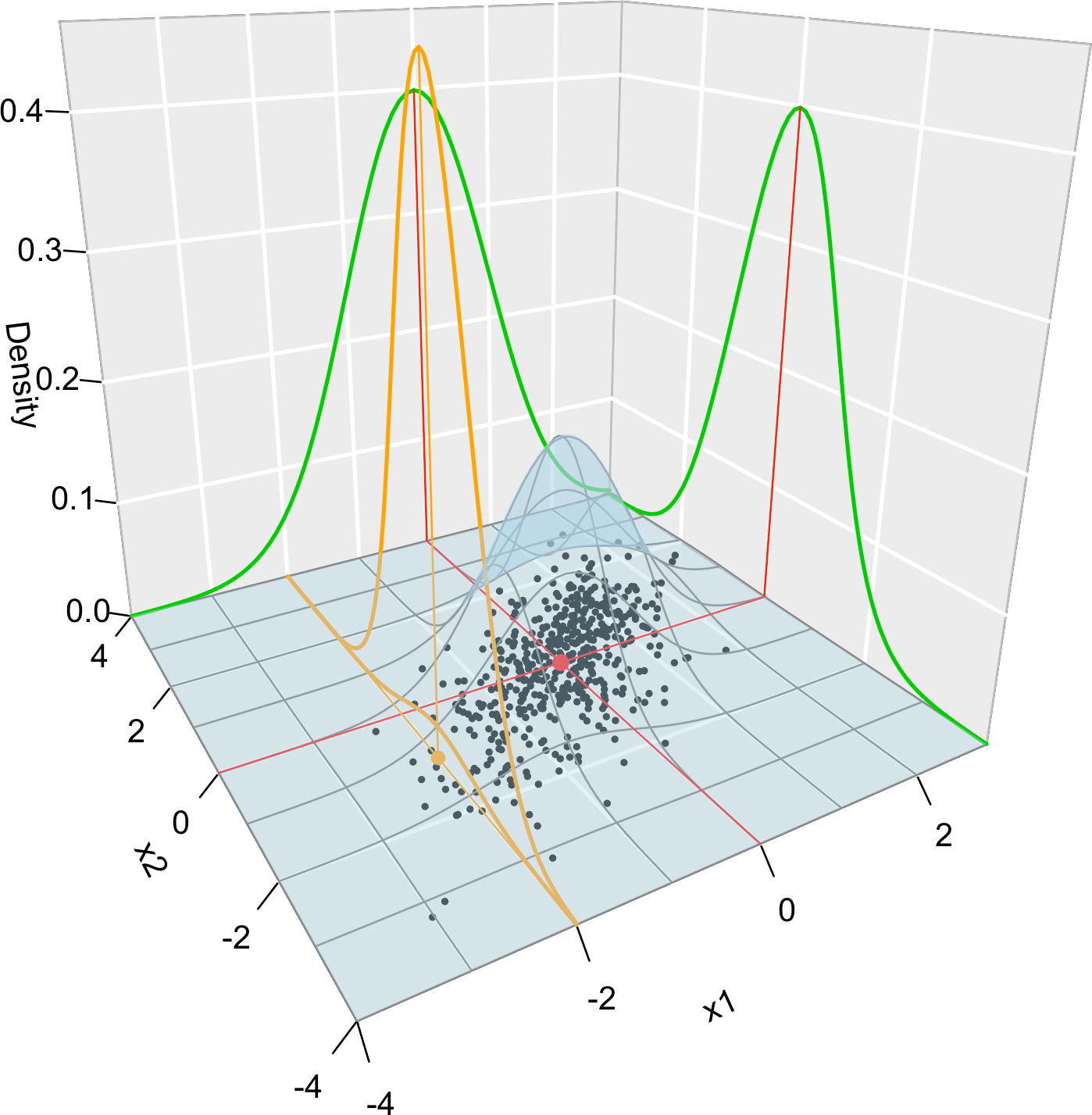
$Visualization of the joint pdf (in blue), marginal pdfs (green), conditional pdf of $X_2| X_1=x_1$ (orange), expectation (red point), and conditional expectation $\mathbb{E}\lbrack X_2 | X_1=x_1 \rbrack$ (orange point) of a $2$-dimensional normal. The conditioning point of $X_1$ is $x_1=-2.$ Note the different scales of the densities, as they have to integrate one over different supports. Note how the conditional density (upper orange curve) is not the joint pdf $f(x_1,x_2)$ (lower orange curve) with $x_1=-2$ but a rescaling of this curve by $\frac{1}{f_{X_1}(x_1)}.$ The parameters of the $2$-dimensional normal are $\mu_1=\mu_2=0,$ $\sigma_1=\sigma_2=1$ and $\rho=0.75.$ $500$ observations sampled from the distribution are shown as black points.$

Figure 1.10: Visualization of the joint pdf (in blue), marginal pdfs (green), conditional pdf of $X_2| X_1=x_1$ (orange), expectation (red point), and conditional expectation $\mathbb{E}\lbrack X_2 | X_1=x_1 \rbrack$ (orange point) of a $2$-dimensional normal. The conditioning point of $X_1$ is $x_1=-2.$ Note the different scales of the densities, as they have to integrate one over different supports. Note how the conditional density (upper orange curve) is not the joint pdf $f(x_1,x_2)$ (lower orange curve) with $x_1=-2$ but a rescaling of this curve by $\frac{1}{f_{X_1}(x_1)}.$ The parameters of the $2$-dimensional normal are $\mu_1=\mu_2=0,$ $\sigma_1=\sigma_2=1$ and $\rho=0.75.$ $500$ observations sampled from the distribution are shown as black points.

Why the apostrophe $'$ in $(X_1(\omega),\ldots,X_p(\omega))'$? This is to indicate that $(X_1(\omega),\ldots,X_p(\omega)),$ a row matrix, has to be transposed, so that it becomes the column matrix $\begin{pmatrix}X_1(\omega)\\\vdots\\X_p(\omega)\end{pmatrix}.$ Vectors are almost always understood in mathematics as column matrices, which is inconvenient for displaying. It is easy to run into inconsistent matrix multiplications if one does not honor the column layout of vectors via the transpose operator.↩︎
That is, $\lim_{\boldsymbol{x}\to\boldsymbol{a}+} F_{\boldsymbol{X}}(\boldsymbol{a})=F(\boldsymbol{a}),$ for all $\boldsymbol{a}\in\mathbb{R}^p.$↩︎
“Almost all” meaning that we exclude a finite or countable number of points and “zero-measure” sets. Zero-measure sets are those with a lower dimension than $p$ (e.g., a curve in $\mathbb{R}^2$).↩︎
Observe $\int_{(a_1,b_1)\times\stackrel{p}{\cdots}\times(a_p,b_p)} f_{\boldsymbol{X}}(\boldsymbol{t})\,\mathrm{d}\boldsymbol{t}=\int_{a_1}^{b_1}\stackrel{p}{\cdots}\int_{a_p}^{b_p} f_{\boldsymbol{X}}(\boldsymbol{t})\,\mathrm{d}t_p\cdots\,\mathrm{d}t_1.$↩︎
Or random vector.↩︎
Observe that the two parameters of this probability model are precisely its expectation vector and variance-covariance matrix. Not all the probability models have parameters relating so neatly with these two concepts!↩︎