Problem Set 5
Problem Set Due Wednesday December 6th at 7pm on Canvas.
For this problem set you will hand in a .Rmd file and a knitted html output.
Please make life easy on us by using sections to clearly delineate questions and sub-questions.
Comments are not mandatory, but extra points will be given for answers that clearly explains what is happening and gives descriptions of the results of the various tests and functions.
Reminder: Put only your student number at the top of your assignment, as we will grade anonymously.
Collaboration on problem sets is permitted. Ultimately, however, the code and answers that you turn in must be your own creation. You can discuss coding strategies, code debugging, and theory with your classmates, but you should not share code or answers in any way.
Please write the names of any students you worked with at the top of each problem set.
Question 1
Load in the file acs, which contains demographic information on every country. This dataset also includes the columns cases.per.1000, which gives the total number of COVID cases per 1000 residents recorded in that county on April 30, 2020.
library(rio)
acs <- import("https://github.com/marctrussler/IIS-Data/raw/main/ACSCountyCOVIDData.Rds")- Plot the bivariate relationship between
percent.transit.commuteon the x-axis andcases.per.1000on the y-axis. Describe what you find.
plot(acs$percent.transit.commute ,acs$cases.per.1000)
The data is heavily skewed. Many counties have very low COVID case numbers per-capita, and many counties have very low level of transit commuting. That being said there appears to be a positive relationship between these two variables.
- Estimate the bivariate regression: \(\hat{Cases.per.1000} = \hat{\alpha} + \hat{\beta_{t}Perc.Transit_i}\). Evaluate and explain the intercept and \(\hat{\beta_{t}}\). Interpret the hypothesis test being performed for \(\hat{\beta_{t}}\).
m1 <- lm(cases.per.1000 ~ percent.transit.commute, data=acs)
summary(m1)
#>
#> Call:
#> lm(formula = cases.per.1000 ~ percent.transit.commute, data = acs)
#>
#> Residuals:
#>     Min      1Q  Median      3Q     Max
#> -12.781  -1.094  -0.735   0.046  58.222
#>
#> Coefficients:
#>                         Estimate Std. Error t value
#> (Intercept)              1.13297    0.05609   20.20
#> percent.transit.commute  0.37685    0.01707   22.08
#>                         Pr(>|t|)
#> (Intercept)               <2e-16 ***
#> percent.transit.commute   <2e-16 ***
#> ---
#> Signif. codes:
#> 0 '***' 0.001 '**' 0.01 '*' 0.05 '.' 0.1 ' ' 1
#>
#> Residual standard error: 3 on 3139 degrees of freedom
#>   (1 observation deleted due to missingness)
#> Multiple R-squared:  0.1344, Adjusted R-squared:  0.1342
#> F-statistic: 487.5 on 1 and 3139 DF,  p-value: < 2.2e-16
The intercept shows that the average number of COVID cases per 1000 people in counties with no transit commuters is 1.13. For every additional percentage point of transit commuters in a county, the number of COVID cases per capita increases by .37. The p-value on this coefficient is very small. There is less than a 1% chance of seeing a regression coefficient this extreme if there was no relationship between transit commuting and COVID in the population.
- In words: why might this relationship between transit commuting and COVID cases be misleading?
Counties with high and low numbers of transit commuters are not very similar. Ideally we would be able to randomly assign the amount of transit commuters to counties and see how that affects COVID cases. Instead, we have a situation where there are potential third variables that cause both the number of transit commuters and COVID cases. Taking into account these third variables may cause us to change our interpretation of the effect of transit commuting on COVID.
- Look in the data set for a variable that might be an omitted variable for the regression in (b) (there is not one answer here), why does variable meet the criteria? Use correlation to show it meets the minimum criteria to be an omitted variable.
I am going to look at the percent of those with a college degree. I want to find a variable that plausibly causes both a high number of transit riders and worse COVID outcomes. Counties with a higher number of people with a college degree are more likely to have a robust transit system. Counties with a college degree may also do a better job of mitigating the impact of COVID and have fewer cases.
I am not worried about post-treatment bias here because it is unlikely that taking public transportation will make someone get a college degree
I can use correlation to confirm that adult poverty rates are related to both transit ridership and covid cases:
cor(acs$percent.college, acs$cases.per.1000, use="pairwise.complete")
#> [1] 0.1073942
cor(acs$percent.college, acs$percent.transit.commute, use="pairwise.complete")
#> [1] 0.3691154
These variables are related, but the expected direction of the relationship of percent college and cases per 1000 is wrong! Counties with more college educated people had more COVID cases early on. (Likely due to international travel).
- Now re-estimate the regression from (b) and add in your proposed omitted variable. Interpret the intercept and the two slope coefficients. How did the coefficient on \(\hat{\beta_{t}}\) change?
m2 <- lm(cases.per.1000 ~ percent.transit.commute + percent.college, data=acs)
summary(m2)
#>
#> Call:
#> lm(formula = cases.per.1000 ~ percent.transit.commute + percent.college,
#>     data = acs)
#>
#> Residuals:
#>     Min      1Q  Median      3Q     Max
#> -12.811  -1.093  -0.731   0.078  58.091
#>
#> Coefficients:
#>                          Estimate Std. Error t value
#> (Intercept)              1.359681   0.137028   9.923
#> percent.transit.commute  0.389133   0.018358  21.197
#> percent.college         -0.011067   0.006104  -1.813
#>                         Pr(>|t|)
#> (Intercept)               <2e-16 ***
#> percent.transit.commute   <2e-16 ***
#> percent.college           0.0699 .
#> ---
#> Signif. codes:
#> 0 '***' 0.001 '**' 0.01 '*' 0.05 '.' 0.1 ' ' 1
#>
#> Residual standard error: 2.999 on 3138 degrees of freedom
#>   (1 observation deleted due to missingness)
#> Multiple R-squared:  0.1353, Adjusted R-squared:  0.1348
#> F-statistic: 245.6 on 2 and 3138 DF,  p-value: < 2.2e-16
The intercept shows that the average number of COVID cases per 1000 people in counties with no transit commuters and no college graduates is is 1.35. Holding constant the percent of residents with a college degree, for every additional percentage point of transit commuters in a county, the number of COVID cases per 1000 residents increases by .39 Holding constant the percent of residents commuting by transit, for every additional percent of the county who has a college degree the impact of COVID drops by .01 per 1000 residents.
- Determine if the coefficient on \(\hat{\beta_{t}}\) from the regression in (b) is statistically distinct from the coefficient on \(\hat{\beta_{t}}\) in part (e) using the bootstrap.
acs.b <- acs[c("cases.per.1000","percent.transit.commute","percent.college")]

coef.diff <- rep(NA, 10000)
for(i in 1:10000){
  bs.data <- acs.b[sample(1:nrow(acs.b), nrow(acs.b), replace=T),]
  m1 <- lm(cases.per.1000 ~ percent.transit.commute, data=bs.data)
  m2 <- lm(cases.per.1000 ~ percent.transit.commute + percent.college, data=bs.data)
  coef.diff[i] <- coef(m2)["percent.transit.commute"] - coef(m1)["percent.transit.commute"]
}

quantile(coef.diff, .025)
#>         2.5%
#> -0.001775106
quantile(coef.diff, .975)
#>      97.5%
#> 0.03404167
No, this difference is not statistically distinguishable from zero. (Answer will change based on variable chosen. )
Question 2
Copy in the following code to generate two related variables, x and y:
- Plot the bivariate relationship between these two variables and estimate the regression of
xpredictingy.
plot(x,y)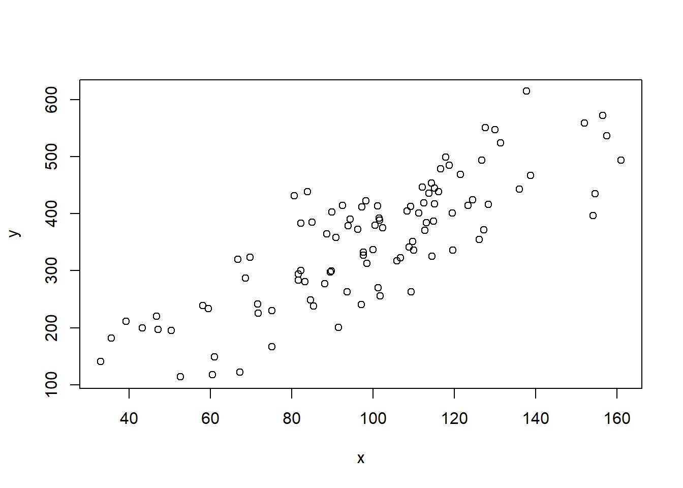
summary(lm(y~x))
#>
#> Call:
#> lm(formula = y ~ x)
#>
#> Residuals:
#>      Min       1Q   Median       3Q      Max
#> -130.269  -40.388    0.677   44.173  139.803
#>
#> Coefficients:
#>             Estimate Std. Error t value Pr(>|t|)
#> (Intercept)  36.6814    23.4249   1.566    0.121
#> x             3.1814     0.2273  13.996   <2e-16 ***
#> ---
#> Signif. codes:
#> 0 '***' 0.001 '**' 0.01 '*' 0.05 '.' 0.1 ' ' 1
#>
#> Residual standard error: 63.47 on 98 degrees of freedom
#> Multiple R-squared:  0.6666, Adjusted R-squared:  0.6631
#> F-statistic: 195.9 on 1 and 98 DF, p-value: < 2.2e-16- Using the above code, repeatedly re-sample these two variables and generate a sampling distribution of the slope coefficient for the regression of x on y. Plot this sampling distribution, and report the standard error.
coef <- rep(NA,10000)
for(i in 1:10000){
  x <- rnorm(100,100,30)
  y  <- 50 + 3*x + rnorm(100, sd=60)
  m <- lm(y~x)
  coef[i] <- coef(m)["x"]
}

plot(density(coef), main="Sampling Distirbution of Beta")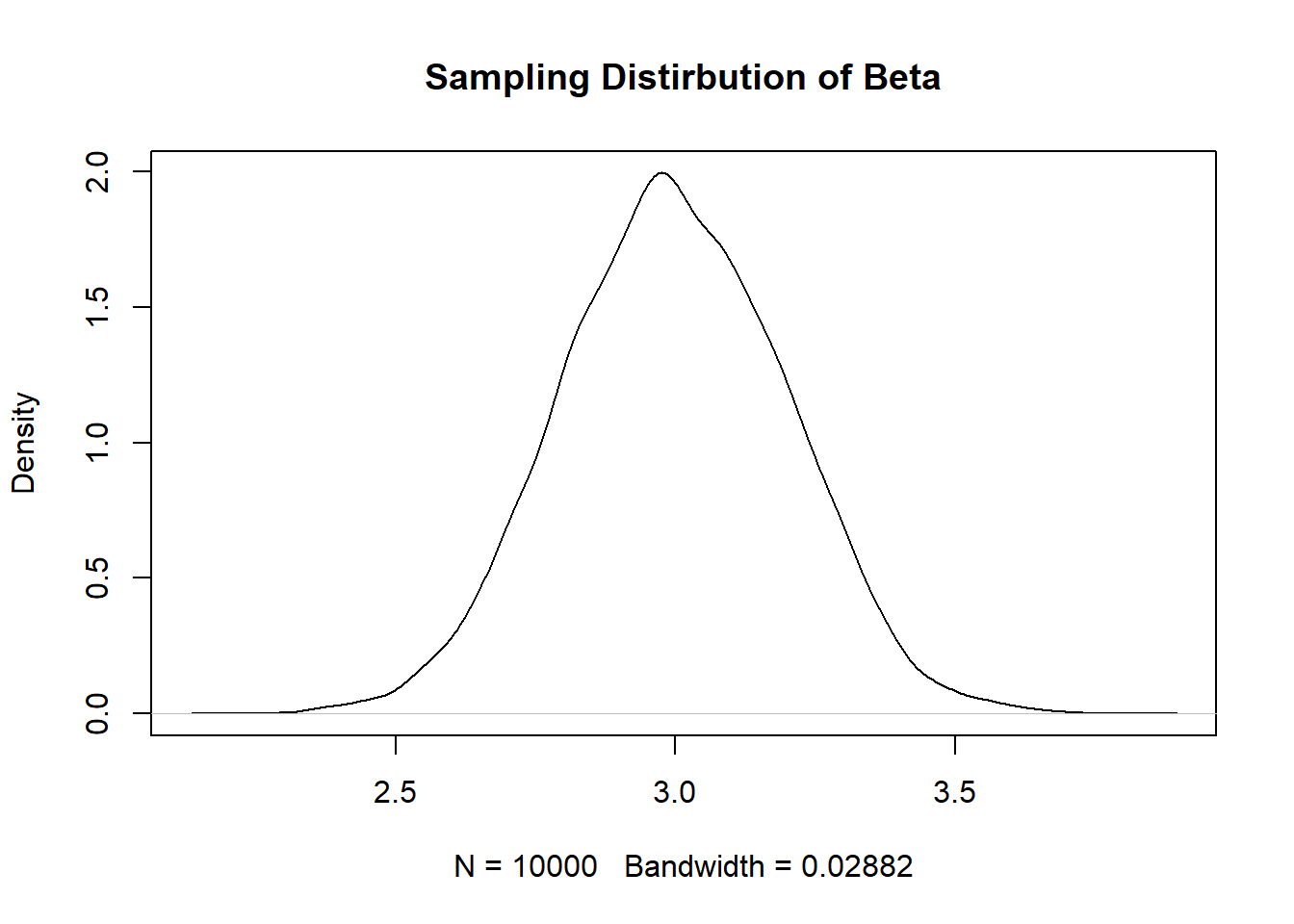
#Standard Error
sd(coef)
#> [1] 0.2020229- What if we want to generate a smaller standard error? Edit the above code in 2 distinct ways that will produce a smaller standard error. Re-sample the data a large number of times, plot the sampling distribution, and report the standard error to show that each change did indeed produce a smaller standard error. (To be clear, you need to make one change, re-sample, and show you have a smaller standard error. Then make a second, distinct, change, re-sample, and show that also produces a smaller standard error.) Reference the equation for the standard error of a regression coefficient to explain why your 2 changes worked.
Three possible changes to make:
Increase the n
coef <- rep(NA,10000)
for(i in 1:10000){
  x <- rnorm(500,100,30)
  y  <- 50 + 3*x + rnorm(100, sd=60)
  m <- lm(y~x)
  coef[i] <- coef(m)["x"]
}

plot(density(coef), main="Sampling Distirbution of Beta")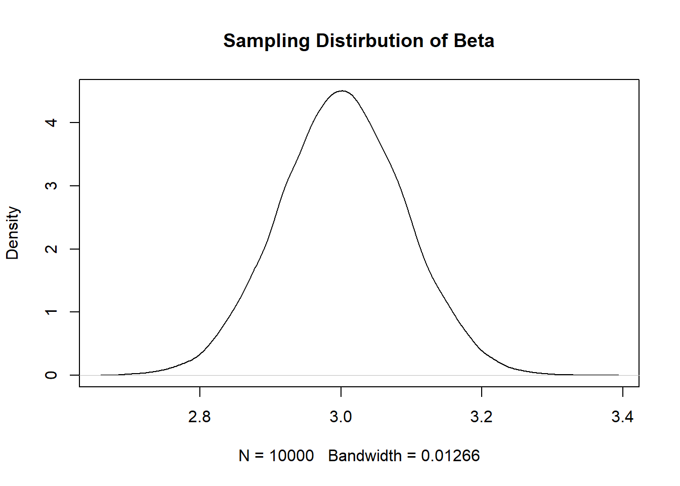
#Standard Error
sd(coef)
#> [1] 0.08873416
Increase the variance in x:
coef <- rep(NA,10000)
for(i in 1:10000){
  x <- rnorm(100,100,60)
  y  <- 50 + 3*x + rnorm(100, sd=60)
  m <- lm(y~x)
  coef[i] <- coef(m)["x"]
}

plot(density(coef), main="Sampling Distirbution of Beta")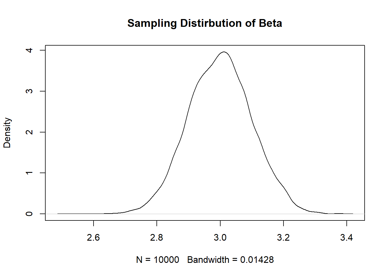
#Standard Error
sd(coef)
#> [1] 0.1001309
Decrease the variance in y:
coef <- rep(NA,10000)
for(i in 1:10000){
  x <- rnorm(100,100,30)
  y  <- 50 + 3*x + rnorm(100, sd=30)
  m <- lm(y~x)
  coef[i] <- coef(m)["x"]
}

plot(density(coef), main="Sampling Distirbution of Beta")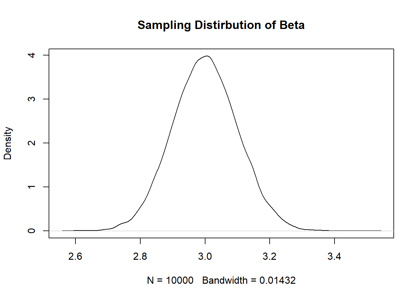
#Standard Error
sd(coef)
#> [1] 0.1003701
The equation for the standard error of a regression coefficient is:
\[ SE_{\beta} = \sqrt\frac{\frac{1}{n} \hat{u_i^2}}{\sum_{i=1}^{n} (X_i - \bar{X})^2} \]
Increasing the N works to reduce this equation through two routes: first there is directly an \(n\) in the numerator that, when larger, will reduce the numerator and thus the standard error. Second, because the denominator does not have an \(n\), additional units will necessarily mean a higher amount of variation from the mean, which will reduce the denominator.
Increasing the variance in \(X\) decreases the standard error because the average deviation of \(x_i\) from \(\bar{x}\) will be higher and thus the denominator will be larger.
Decreasing the variance in \(y\) decreases the standard error because, all else equal, it will reduce the potential size of the errors made in the regression, and thus reduce the numerator of the equation.