15 Final Review
15.1 The Big Picture
The fundamental task of statistics is not to describe the dataset in front of us but instead to make inferences about the population from which the sample is drawn.
The parts of this course where we estimated something from our dataset were relatively straightforward. How do you get a mean? How do you measure covariance? How do you turn that covariance into a correlation or a regression coefficient? The math for all of those things are pretty straightforward, and when it’s not (we didn’t do the matrix algebra for multiple regression) the interpretation was straightforward.
The more conceptually difficult part of this course (and the part that I want you to think about when you think about this course) was conceptualizing each and every thing that we estimate in a data set as an infinite number of possible estimates we could get from an infinite number of data sets that could exist. Critically (and magically!) the distribution of all of those possible estimates from all those possible datasets is predictable.
Everything we estimate in one data set has a sampling distribution and a standard error which allow us to make inferences about the population. These inferences are what statistics is about
Consider an example I used in the first class. Here is the distribution of the feeling thermometer question on Donald Trump from the 2020 ANES
library(rio)
anes <- import(file="https://raw.githubusercontent.com/marctrussler/IIS-Data/main/ANES2020Clean.csv")

plot(density(anes$therm.trump,na.rm=T), xlim=c(0,100), main="Distribution of Trump Themometer Ratings")
abline(v=mean(anes$therm.trump,na.rm=T), lty=2)
legend("topright", c(paste("Mean = ",round(mean(anes$therm.trump,na.rm=T),2 )),
                     paste("SD = ",round(sd(anes$therm.trump,na.rm=T),2 )) ), lty=2, col=c("Black", "White"))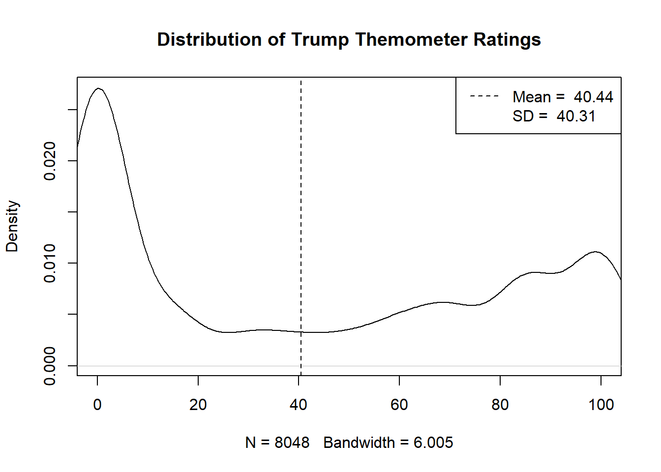
Here’s what I said at the time:
We can also summarize the distribution of this variable in the sample with summary statistics. The mean – or simple average – of this variable, for example, is 40.44. The standard deviation – which can be thought of as how much each individual deviates from the mean, on average – is 40.31.
The problem is, that’s not at all what we care about. What we care about, in the example of a Trump feeling thermometer, is how all voters in the feel about Trump, not just the ones in this sample. What is the true average feeling towards Trump amongst all voters? How spread out is that opinion? Do the opinions of Democrats and Republicans differ? All of these questions are not immediately or obviously answered by the data in front of us.
It is tempting to say: well if this is a sample of data from the population isn’t the answer the same in the population? Isn’t it good enough to get a sample, report what’s in that sample, and assume it’s the same as the population?
To some degree our answer to this is actually, yes! But let’s think for a little bit: if we took another sample of 8000 Americans would this plot look exactly the same? How much could we expect it to vary? It obviously will not be exactly the same…. so how do we know that this distribution is the one that is representative of the population?
We now have a lot of insight into all of these questions. After studying for the final you should have a good sense of why it is that we have good insights into those questions!
15.2 Standard Error of the Mean
We care about three distributions: a population, a sample, and the sampling distribution of an estimate we form using out sample.
This is true no matter what we are estimating but it is simplest to think about in terms of the mean.
First is the population that we are sampling from. Somthing like this.
eval <- seq(-5,60,.001)
plot(eval,dchisq(eval,10,ncp=12), type="l", main="Population",
     xlab="Values",ylab="Density", ylim=c(0,0.06), xlim=c(0,65))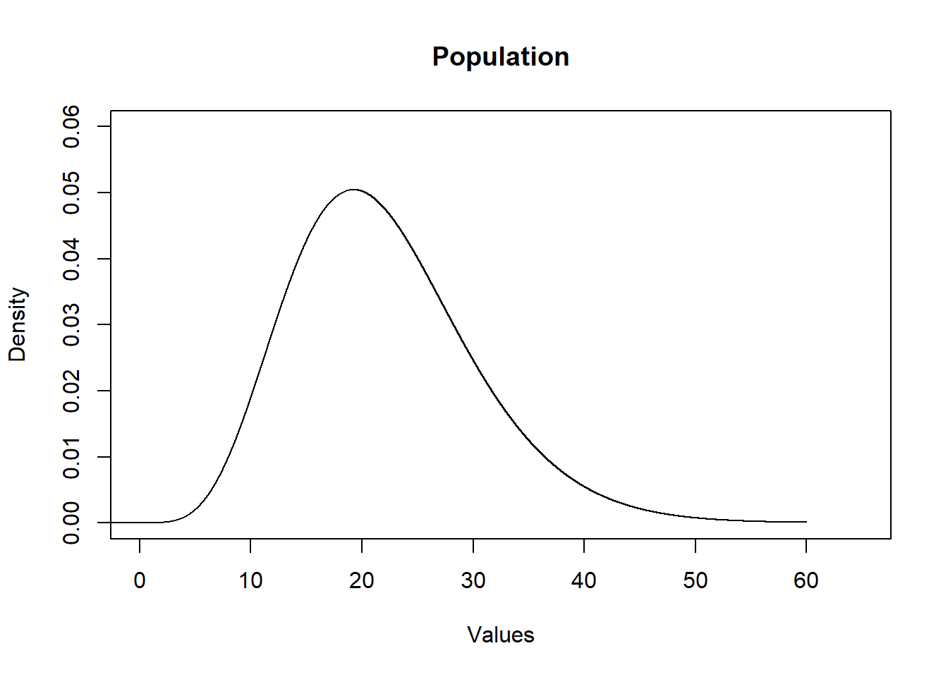
We can think of the population as the “Data Generating Process”. It can be anything.
The second distribution we care about is the sample we get from this population:
set.seed(19104)
x <- rchisq(50,10,ncp=12)
head(x)
#> [1] 17.17206 15.50880 29.22219 18.31710 31.47061 20.98213
plot(density(x), main="Sample", xlab="Value", ylim=c(0,0.06), xlim=c(0,65))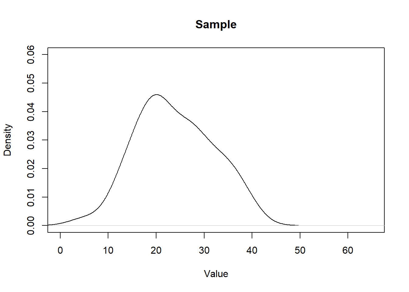
We can think of each sample as being a rough approximation of the population it was generated from. The larger the sample size, the more the sample will look like the population. (However, critically, this is NOT what the Central Limit Theorem is.)
Here are the two distributions side-by-side:
plot(density(x), main="Sample", xlab="Value", ylim=c(0,0.06), xlim=c(0,65))
points(eval,dchisq(eval,10,ncp=12),col="firebrick", type="l")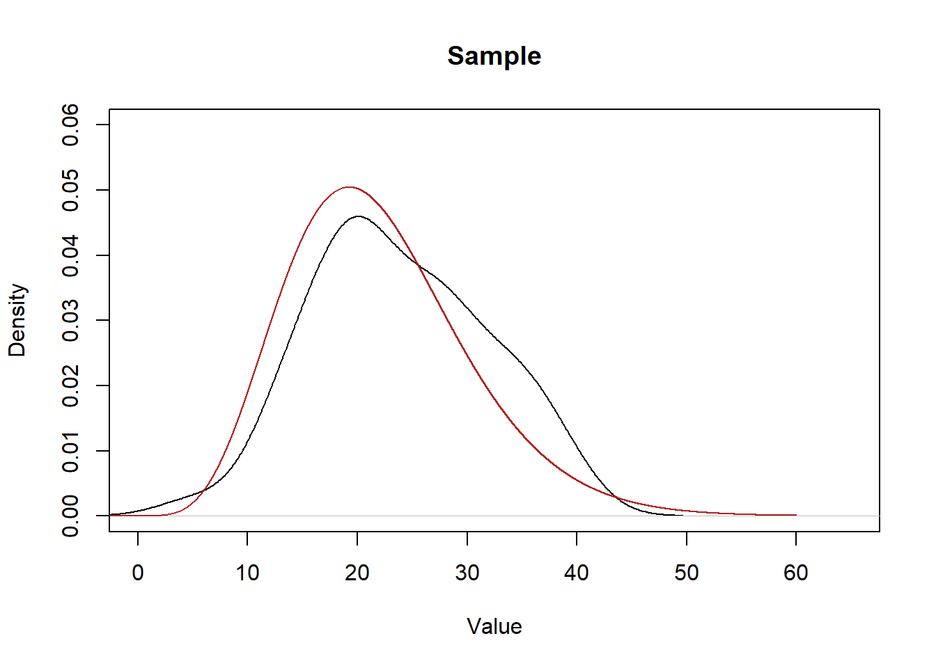
Every time we take a sample we will get a distribution of data that will be a rough approximation of the population.
The key thing we learned before the midterm is, while it’s somewhat futile to ask “How much will my sample distribution look like the population for a sample size of \(n\)?”, we can predict how much the sample mean will look like the true population expected value.
Because of the central limit theorem We know that the sample mean is itself a random variable, with this distribution \(\bar{X_n} \sim N(\mu=E[X], \sigma^2 = V[X]/n)\).
Specifically, each sample mean for an n of 50 will be drawn from this normal distribution, based on my knowledge that the \(E[X]=22\) and \(V[X]=68\).
mean.eval <- seq(15,29,.001)
plot(mean.eval, dnorm(mean.eval, mean=22, sd=sqrt(68/50)), type="l",
     main="Sampling Distribution of the Sample Mean",
     xlab="Value of Sample Mean",
     ylab="Density")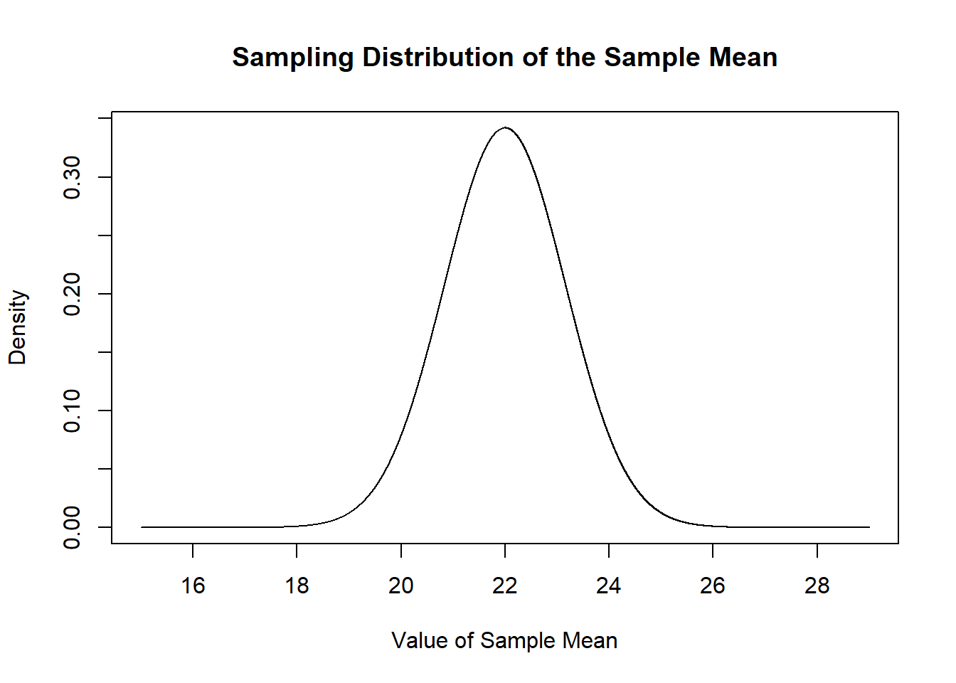
We can prove this to ourselves by repeatedly sampling and taking a bunch of sample means and plotting their density compared to this sampling distribution.
sample.means <- rep(NA, 10000)

for(i in 1:10000){
  sample.means[i] <- mean(rchisq(50,10,ncp=12))
}

plot(mean.eval, dnorm(mean.eval, mean=22, sd=sqrt(68/50)), type="l",
     main="Sampling Distribution of the Sample Mean",
     xlab="Value of Sample Mean",
     ylab="Density")
points(density(sample.means), type="l", col="darkblue")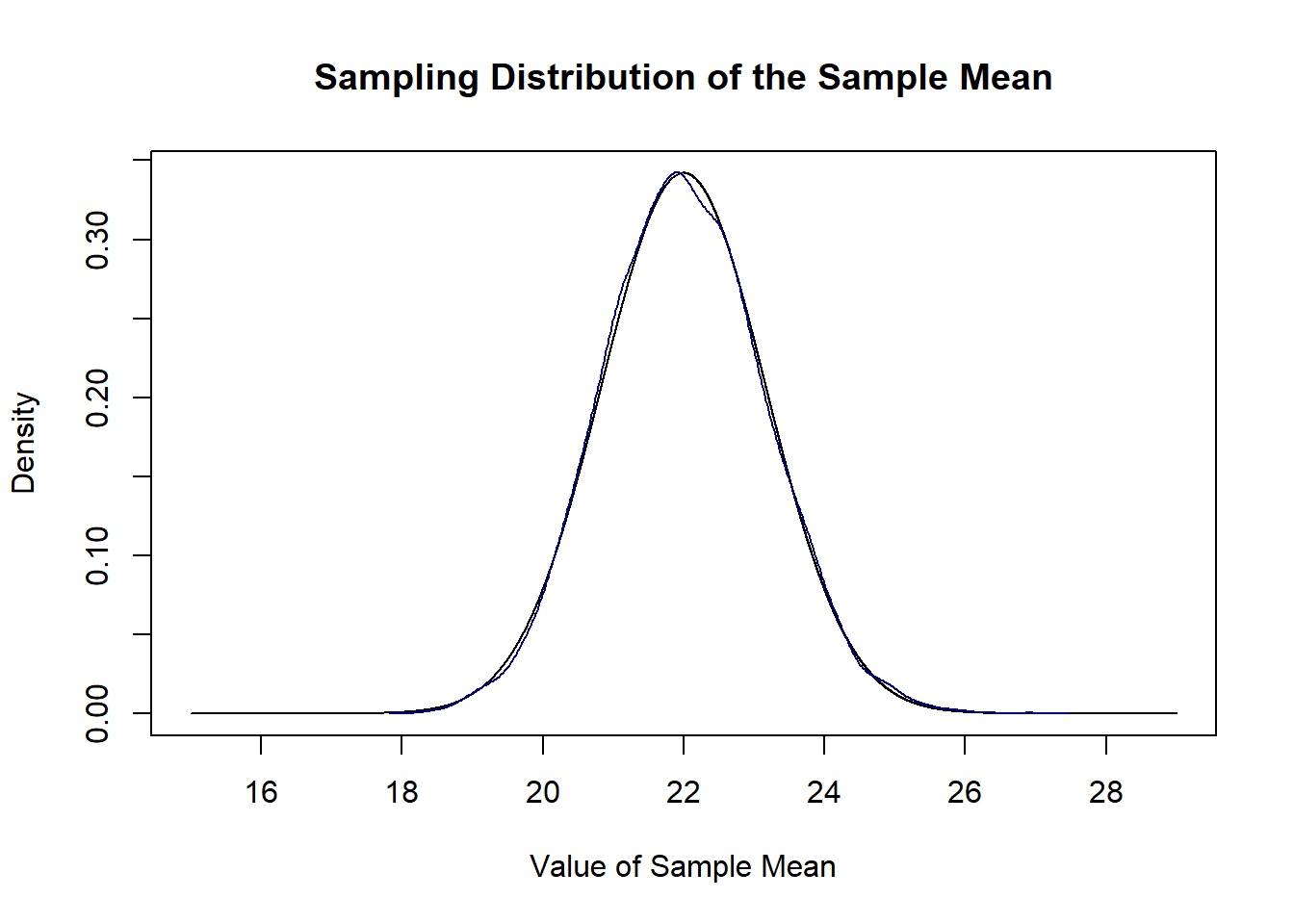
They are the same distribution. Because this sampling distribution is normally distributed it is easy to determine the probability falling in certain ranges.
15.2.1 But we don’t know the population variance
Our definition of the sampling distribution made use of \(V[X]\) the population level variance. But we don’t have that!
Instead, we make use of the sample standard deviation as a stand in for \(\sqrt{V[X]}\).
When we are using the sample standard deviation as a stand in for the population variance in the calculation of the standard error, however, the sampling distribution of the sample mean is t distributed with \(n-1\) degrees of freedom. This really only affects sample sizes under 30, but still, it is theoretically important that the sample mean is \(t\) distributed not distributed standard normal.
\[ \frac{\bar{X_n}-E[X]}{s/\sqrt{n}} \sim t_{n-1} \]
15.2.2 Confidence Intervals
We define a confidence level as \((1-\alpha)*100\), such that a 70% confidence interval implies an \(\alpha\) of .3.
For a given \(\alpha\) a confidence interval around any given sample mean is:
\[CI(\alpha) = [\bar{X_n}-t_{\alpha/2}*SE,\bar{X_n}+t_{\alpha/2}*SE]\]
If we had \(\bar{x}=3\), \(s=2\), \(n=100\) and want to find a 95% confidence interval the steps are:
Derive the standard error:
se <- 2/sqrt(100)Determine how many standard errors puts \(\alpha/2=.05/2=.025\) probability mass in the left tail in the \(t\) distribution with 99 degrees of freedom:
t <- qt(.975, df=99)Now plug these values into the above equation:
c(3-t*se, 3+t*se)
#> [1] 2.603157 3.396843
The interpretation of a confidence interval comes from the fact that if we repeatedly re-sample and form confidence intervals, 95% of them will contain the true population paramater.
The fully correct interpretation is: 95% of similarly constructed confidence intervals will contain the true population paramter.
The technically incorrect, but good enough for me, interpretation is: there is a 95% chance this confidence interval contains the true population paramter.
15.3 Hypothesis Tests
The logic of hypothesis testing comes from the fact that we don’t know where the sampling distribution of an estimate is centered, but we feel that we have a good sense of it’s shape (via the CLT).
So we have this normal distribution and need to put it somewhere. All we are doing with a hypothesis testing is positing that the sampling distribution is centered on the null hypothesis and determining how likely it is to get the result we got in our sample under that assumption.
The five steps to a hypothesis test are:
- Specify a null hypothesis and an alternative hypothesis.
- Choose a test statistic and the level of test (\(\alpha\)).
- Derive the sampling distribution and center on the null hypothesis.
- Compute the p-value (one sided or two sided).
- Reject the null hypothesis if the p-value is less than or equal to \(\alpha\). Otherwise retain the null hypothesis.
If we had this sample:
#We don't care about the population it comes from
set.seed(19103)
x <- rnorm(1000, 0.2, 3)

mean(x)
#> [1] 0.1536556
sd(x)
#> [1] 2.968243
And wanted to test the null hypothesis that \(\mu=0\) and the alternative hypothesis that \(\mu \neq 0\) we could approximate the sampling distribution under the null hypothesis as:
se <- sd(x)/sqrt(1000)
eval <- seq(-.5,.5, .001)

plot(eval, dnorm(eval, mean=0, sd=se), type="l", main="Sampling Distribution Under the Null")
abline(v=mean(x))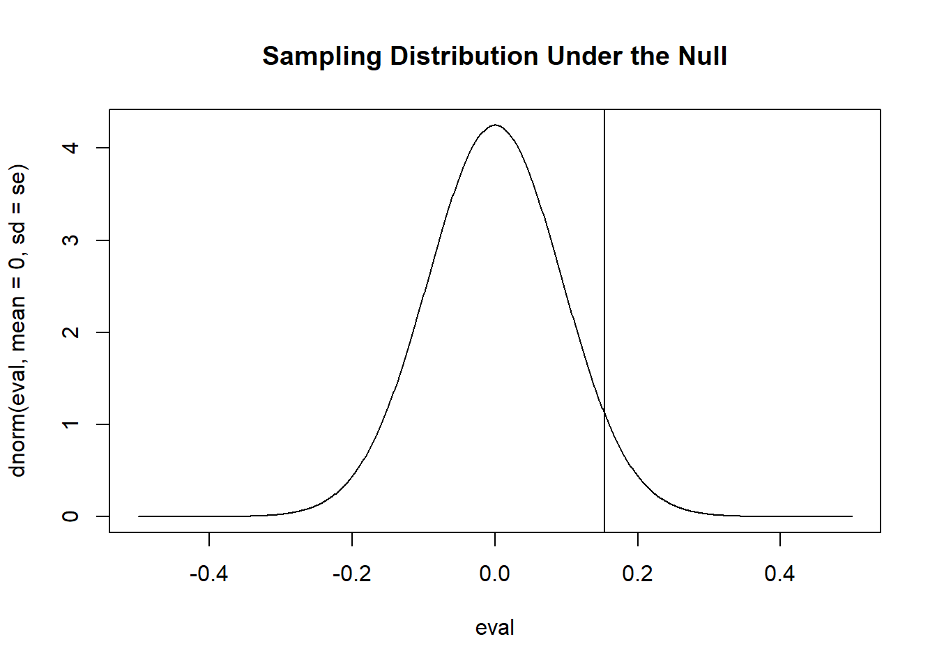
“Approximate” because I am using a normal distribution to visualize this as I calculated the standard error using the sample standard deviation, so this sampling distribution should be t-distributed.
We are going to set an \(\alpha=.05\) which means we want there to be a 5% or lower probability of false positive. In terms of our figure that means we want to put 5% of the probability mass in the tails and 95% of the probability mass in the center.
plot(eval, dnorm(eval, mean=0, sd=se), type="l", main="Sampling Distribution Under the Null")
abline(v=qnorm(c(.025,.975), mean=0, sd=se), lty=2, col="firebrick")
abline(v=mean(x))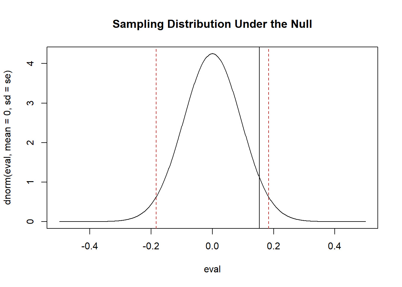
If this is the true sampling distribution, there is a 5% of producing means to the left and right of those two red lines (in the tails). If our mean is in that range, there is less than 5% chance of getting a result that extreme simply by chance. This is why we reject the null hypothesis if our mean is in that range. In this case our mean is not in that range. There is a higher than 5% of producing a mean at least that extreme under this distribution. So we fail to reject the null hypothesis.
To calculate a p-value for a two-tailed test we want to add up the probability mass in the tail that is to the right of our sample mean as well as the probability mass to the left of our mean once it is flipped to the other side of the null. Because the normal distribution is symmetrical we can just find one of these values and multiply by 2.
The p-value is around 10%. Greater than our 5% threshold, as expected.
Now we know that this is technically t-distributed. So to skip all the above visualizations I can just evaluate: how many standard errors away from the null is my mean, and what does that mean in the t distribution?
Those last two steps are all we really need to do for a hypothesis test. The rest of the above is just to help us visualize. You should really understand those last two steps.
The other part of hypothesis testing that is critical to understand is: all of the things we have estimated in this class have a normal or t distribution. Once you have a standard error (and a degrees of freedom if t-distributed) you can do the hypothesis test. It doesn’t matter if that’s a mean, or a difference in means, or a regression coefficient, or a marginal effect….
15.3.1 Power
The level of our statistical test, \(\alpha\), is the probability of a false positive. If we think about a drug trial, this is the accepted risk of saying a drug works when it does not work. We want this to be very low because science is inherently conservative. Helpfully, we get to just set this level as part of our hypothesis test.
More tricky is \(\beta\) the probability of a false negative. Again thinking about a drug trial, this is the the probability of saying a drug doesn’t work when it actually does. We don’t get to set \(\beta\). The things that determine it are (1) the width of our sampling distribution and the difference between the truth and the null hypothesis.
The two things you have to think about when calculating power are:
Given my standard error and null hypothesis, what is the range of values where I will fail to reject the null hypothesis?
Given my standard error and assumption (or knowledge) of the truth of the population parameter, what range of estimates will be produced?
Then you need to determine how many of the estimates produced by (2) will end up in the range defined by (1).
So, taking the variable x above, we had:
In this case I know that the true population mean is 0.2 and the true population standard deviation is 3 (or \(V[X]=9\)). That means the sampling distribution of the sample mean will be \(\sqrt{9/1000} = .095\).
So we have a standard error, we have a truth (0.2), and let’s assume that our null hypotehsis test is still \(\mu=0\).
We don’t have to visualize this, though I have been to help you see what i’m talking about. But to just quickly do the math:
Here is the range of values where we will fail to reject the null hypothesis:
Now determine the probability of drawing means in that zone, given the truth:
There is about a 44% chance of drawing a mean that will fall into the zone where we will mistakenly fail to reject the null hypothesis. This is a high probabiliy of a false negative and therefore a low amount of power.
In the case where we know the data generating process (i.e. I can see the rnorm command that is generating data, we can simulate to get the same answer):
15.4 Bootstrap
There are four ways to calculate a sampling distribution (and therefore, a standard error):
- You have information about the population that allows you to calculate a standard error.
For example, in situations where I told you that the population level \(V[X]\).
- You know the population/DGP and repeatedly sample and generate estimates. The result will be a sampling distribution.
This is the literal “sampling distribution” as it is a distribution of a bunch of estimates from a bunch of samples. The standard deviation of this distribution is the standard error.
- You have information about the sample and an equation that produces the standard error.
This is the “standard” situation that allows us to calculate the standard error of the mean for a single sample, but is also how we get the standard error for the difference in means, for a regression coefficient, for a marginal effect. We know how to figure these things out using math.
- Bootstrap
The fourth method is a rough approximation of the second method. Instead of repeatedly re-sampling from a population, we use the fact that our sample is iid to produce the insight that “random samples of our sample are new samples”.
We repeatedly re-sample rows in our data-set, calculate the thing we are estimating in each new “sample”, and produce a sampling distribution. The standard deviation of this sampling distribution will be our estimate of the standard error.
This method is a “last resort”. We would never use this to estimate the standard error of the mean (we have an equation for that!). But we will use this for things that don’t have a standard error like a correlation coefficient, the difference between two correlation coefficients, or two regression coefficients that come from two different models.
15.5 Covariance and Correlation
15.5.1 Difference in means
To extend our knowledge of sampling distributions and hypothesis testing we started to consider the relationships between variables, starting with a situation where we calculated the mean of a variable for two different groups. (We can think about this as the relationship between the variable \(x\) and a group indicator with exactly two values).
We wanted to think about hypotheses like these:
\[ H_o:\mu_c - \mu_t = 0\\ H_a: \mu_c - \mu_t \neq 0 \]
So if we have two means the hypothesis we often want to answer is whether they are equal, or not.
What is critical (in line with our discussion above of sampling distributions and hypothesis tests) is once you have the standard error everything is exactly the same.
Here the standard error is:
\[ se = \sqrt{\frac{\sigma_0^2}{n_0} + \frac{\sigma_1^2}{n_1} } \]
If we have that, an estimate (say a difference in means of….3… or 0.2… it doesn’t really matter) than our hypothesis test (or a power test) continues exactly as it did for a single mean.
I’m not going to make you calculate the degrees of freedom for a difference in means on the exam :)
We can easily perform a difference in means test using the t.test function:
set.seed(19104)
y0 <- rnorm(50,23, 13)
y1 <-  rnorm(50, 28, 6)
y <- c(y0,y1)
x <- c(rep(0,50), rep(1,50))
dat <- cbind.data.frame(x,y)
head(dat)
#>   x        y
#> 1 0 17.85445
#> 2 0 25.55715
#> 3 0 29.99189
#> 4 0 28.97014
#> 5 0 22.22095
#> 6 0 10.75801

#T.test
t.test(dat$y ~ dat$x)
#>
#>  Welch Two Sample t-test
#>
#> data:  dat$y by dat$x
#> t = -3.1014, df = 77.848, p-value = 0.002683
#> alternative hypothesis: true difference in means between group 0 and group 1 is not equal to 0
#> 95 percent confidence interval:
#>  -9.012638 -1.965384
#> sample estimates:
#> mean in group 0 mean in group 1
#>        22.44682        27.93583
Note that we get the same result via regression:
summary(lm(dat$y ~ dat$x))
#>
#> Call:
#> lm(formula = dat$y ~ dat$x)
#>
#> Residuals:
#>      Min       1Q   Median       3Q      Max
#> -27.3657  -5.6623   0.3217   5.3519  25.0263
#>
#> Coefficients:
#>             Estimate Std. Error t value Pr(>|t|)
#> (Intercept)   22.447      1.251  17.936  < 2e-16 ***
#> dat$x          5.489      1.770   3.101  0.00252 **
#> ---
#> Signif. codes:
#> 0 '***' 0.001 '**' 0.01 '*' 0.05 '.' 0.1 ' ' 1
#>
#> Residual standard error: 8.849 on 98 degrees of freedom
#> Multiple R-squared:  0.08938,    Adjusted R-squared:  0.08008
#> F-statistic: 9.619 on 1 and 98 DF,  p-value: 0.002516
15.5.2 Covariation and Correlation
As a bridge to get to regression we thought about the covariation between two variables and the (related) concept of correlation. We need these two things to describe the inter-relationship between two continous variables.
Covariance is defined as:
\[ \hat{\sigma_{x,y}} = \frac{1}{n-1}\sum_{i=1}^n (x_i-\bar{x})(y_i - \bar{y}) \] We add up the deviations of x from it’s mean and multiply by the deviations from y from it’s mean.
Covariation is a critical building block, but it’s major problem is that it doesn’t have clear units. If you multiply x and y by 100 covariation will get much higher, even though it is describing the same relationship.
As such we quickly pivot to correlation, which is just covariation standardized by the variation in the two variables:
The idea behind correlation is simply to standardize a covariance by dividing by the standard deviations of the variables that we are measuring. Specifically, the correlation equals:
\[ \hat{\rho}_{x,y} = \frac{\hat{\sigma}_{x,y}}{\sqrt{var(x)*var(y)}} \]
Correlation ranges from -1 (perfect negative correlation) to 1 (perfect correlation).
15.6 Bivariate Regression
The need to expand on correlation came from two drawbacks. First, the “unitless” character of correlation makes it hard to form real, human, sentences about the size of effects. Second, our ability to consider third (or fourth, or fifth) variables is extremely blunt (i.e. we can maybe look at the correlation in a few subgroups of a third variable, but not much beyond that).
Regression summarizes the relationship between two variables by drawing a line in a two-dimdensional space. Specifically we estimate the following equation:
\[ \hat{y} = \hat{\alpha} + \hat{\beta}x_i \]
Where \(\hat{\alpha}\) is the y-intercept, \(\hat{\beta}\) is the slope, and \(x_i\) is each data-points x value.
For any given value of x, bivariate regression returns the predicted value of y.
The two coefficients, \(\hat{\alpha}\) and \(\hat{\beta}\) are chosen such that they minimize the sum of the squared residuals. Where the residuals are:
\[ \hat{u_i} = y_i - \hat{y} \]
The regression line is the line that minimizes the vertical distance to each data point.
Going through the math to determine what minimizes the sum of the squared residuals, we found that:
\[ \hat{\alpha} = \bar{Y} - \hat{\beta}\bar{x} \]
And
\[ \hat{\beta} = \frac{\sum_{i=1}^n (y_i - \bar{y})(x_i - \bar{x})}{\sum_{i==1}^n(x_i -\bar{x})^2} \\ \]
For this second equation, we also showed that it simplifies to
$$ = \
$$ The covariance of x and y divided by the variance of x. Correlation and Regression are nothing more than the re-scaling of covariation.
We further discussed how to interepret a regression. Consider this regression of age on the blm feeling thermoemter
library(rio)
anes <- import("https://github.com/marctrussler/IIS-Data/raw/main/ANESFinalProjectData.csv")

anes$age <- anes$V201507x
anes$age[anes$age<0] <- NA

anes$blm.therm <- anes$V202174
anes$blm.therm[anes$blm.therm<0 | anes$blm.therm>100] <- NA

m <- lm(blm.therm ~ age, data=anes)
summary(m)
#>
#> Call:
#> lm(formula = blm.therm ~ age, data = anes)
#>
#> Residuals:
#>     Min      1Q  Median      3Q     Max
#> -62.690 -33.381   4.049  32.202  54.049
#>
#> Coefficients:
#>             Estimate Std. Error t value Pr(>|t|)
#> (Intercept) 67.54966    1.32870   50.84   <2e-16 ***
#> age         -0.26998    0.02437  -11.08   <2e-16 ***
#> ---
#> Signif. codes:
#> 0 '***' 0.001 '**' 0.01 '*' 0.05 '.' 0.1 ' ' 1
#>
#> Residual standard error: 35.12 on 7062 degrees of freedom
#>   (1216 observations deleted due to missingness)
#> Multiple R-squared:  0.01709,    Adjusted R-squared:  0.01695
#> F-statistic: 122.8 on 1 and 7062 DF,  p-value: < 2.2e-16
The interpretation of the intercept is always the average value of y when all variables are equal to zero. We can see that this is just mathematically true from the regression equation:
\[ \hat{y} = \hat{\alpha} + \hat{\beta}x_i \\ \hat{y} = \hat{\alpha} + \hat{\beta}*x_i*0 \\ \hat{y} = \hat{\alpha}\\ \]
That may, or may not, be a helpful value. In this case, this is the predicted average blm.therm score for when age is 0. That’s clearly a nonsense number.
The interpretation of \(\beta\) is always how a 1-unit change in the independent variable leads to a \(\beta\) change in the dependent variable. By 1-unit we mean 1-unit in our number system. This is true in EVERY REGRESSION. In this case, 1-unit is a year of aging. So for every additional year a person get’s older we expect their blm.therm to drop by around .27.
The interpretation of regression coefficients therefore completely depends on the scale of the variable. If we instead had age in months, the underlying relationship would be no different, but the coefficient would change it’s value:
anes$age.months <- anes$age*12
m2 <- lm(blm.therm ~ age.months, data=anes)
summary(m2)
#>
#> Call:
#> lm(formula = blm.therm ~ age.months, data = anes)
#>
#> Residuals:
#>     Min      1Q  Median      3Q     Max
#> -62.690 -33.381   4.049  32.202  54.049
#>
#> Coefficients:
#>              Estimate Std. Error t value Pr(>|t|)
#> (Intercept) 67.549664   1.328699   50.84   <2e-16 ***
#> age.months  -0.022498   0.002031  -11.08   <2e-16 ***
#> ---
#> Signif. codes:
#> 0 '***' 0.001 '**' 0.01 '*' 0.05 '.' 0.1 ' ' 1
#>
#> Residual standard error: 35.12 on 7062 degrees of freedom
#>   (1216 observations deleted due to missingness)
#> Multiple R-squared:  0.01709,    Adjusted R-squared:  0.01695
#> F-statistic: 122.8 on 1 and 7062 DF,  p-value: < 2.2e-16
“One unit” is no longer one year, but is now one month. As such the coefficient is much smaller. An individual getting one month older leads to a .022 decline in their blm thermometer score.
If one unit is one month then 12 units is one year. As such we can see:
coef(m2)["age.months"]*12
#> age.months
#> -0.2699798
Multiplying this coefficient by 12 returns the original variable.
15.6.1 The standard error of a regression coefficient
The standard error of a regression coefficient is given by:
\[ SE_{\beta} = \sqrt{\frac{ \frac{1}{n} \sum_{i=1}^n u_i^2 }{\sum_{i=1}^n (x_i-\bar{x})^2} } \]
The average squared residual divided by the sum of the deviations of the x’s from the mean. The counter-intuitive part of this is that the standard error of a regression coefficient gets smaller when x has more variation, which is backwards from a lot of other things.
As discussed throughout this review, once you have a regression coefficient (an estimate) and a standard error, everything about a hypothesis test is the same.
15.7 Multivariate Regression
When we just look at a bivariate regression we might not be uncovering the true effect of x on y.
In particular, we are concerned with omitted variables that are a cause of both x and y.
We can “control” for these additional variables, z, by putting them in our regression.
When z has one or two categories, one way that we can conceptualize of regression is that we are adding seperate intercepts for each category.
For example we looked at how the relationship between the student to teacher ratio in schools and test scores in California schools might be affected by whether a school is a high.esl or low.esl school
## ---------------------------------------------------------
library(AER)
#> Warning: package 'AER' was built under R version 4.1.2
#> Loading required package: car
#> Warning: package 'car' was built under R version 4.1.2
#> Loading required package: carData
#> Warning: package 'carData' was built under R version 4.1.2
#> Loading required package: lmtest
#> Warning: package 'lmtest' was built under R version 4.1.2
#> Loading required package: zoo
#>
#> Attaching package: 'zoo'
#> The following objects are masked from 'package:base':
#>
#>     as.Date, as.Date.numeric
#> Loading required package: sandwich
#> Loading required package: survival
data("CASchools")
CASchools$STR <- CASchools$students/CASchools$teachers
CASchools$score <- (CASchools$read + CASchools$math)/2
dat <- CASchools

## ---------------------------------------------------------
dat$high.esl <-NA
dat$high.esl[dat$english>=median(dat$english)]<- 1
dat$high.esl[dat$english<median(dat$english)]<- 0

## ---------------------------------------------------------
plot(dat$STR, dat$score, xlab="Student:Teacher Ratio", ylab="Test Score", pch=16, type="n")
points(dat$STR[dat$high.esl==0], dat$score[dat$high.esl==0], pch=16, col="darkblue")
points(dat$STR[dat$high.esl==1], dat$score[dat$high.esl==1], pch=16, col="firebrick")
abline(a=691.32, b=-1.3963, col="darkblue", lwd=3)
abline(a=691.32-19.49, b=-1.3963, col="firebrick", lwd=3)
legend("topright", c("Low ESL", "High ESL"), pch=c(16,16), col=c("darkblue", "firebrick"))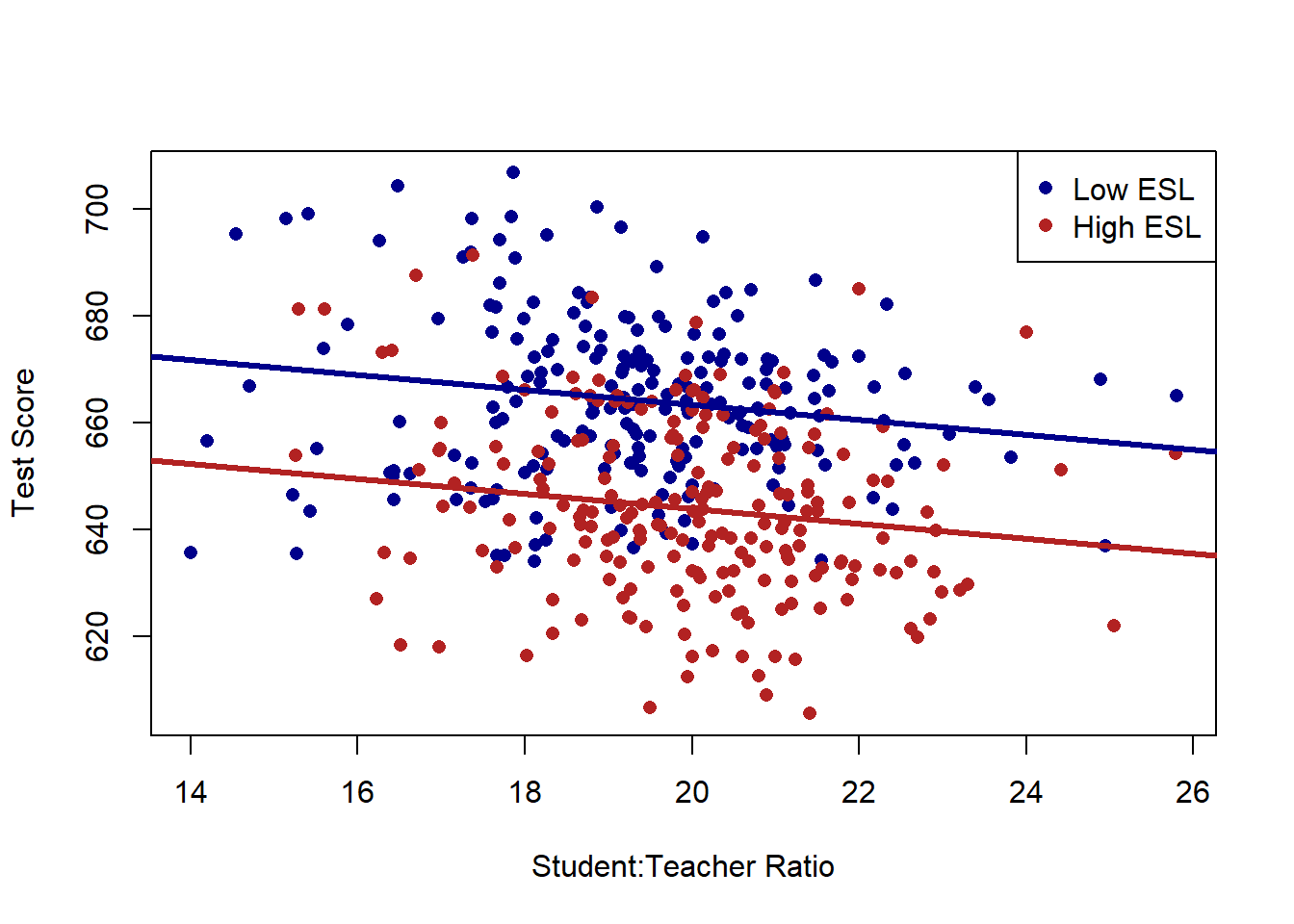
And in particular that some of the negative relationship between classroom size and test scores could be explained by this third variable.
m <- lm(score ~ STR + high.esl, data=dat)
summary(m)
#>
#> Call:
#> lm(formula = score ~ STR + high.esl, data = dat)
#>
#> Residuals:
#>     Min      1Q  Median      3Q     Max
#> -37.857 -10.853  -0.626  10.198  43.834
#>
#> Coefficients:
#>             Estimate Std. Error t value Pr(>|t|)
#> (Intercept) 691.3267     8.1315  85.019  < 2e-16 ***
#> STR          -1.3963     0.4171  -3.348 0.000889 ***
#> high.esl    -19.4911     1.5763 -12.365  < 2e-16 ***
#> ---
#> Signif. codes:
#> 0 '***' 0.001 '**' 0.01 '*' 0.05 '.' 0.1 ' ' 1
#>
#> Residual standard error: 15.91 on 417 degrees of freedom
#> Multiple R-squared:  0.3058, Adjusted R-squared:  0.3025
#> F-statistic: 91.84 on 2 and 417 DF,  p-value: < 2.2e-16
Thinking about how to interpret regression with more than one variable, everything stays exactly the same. The intercept is still the average value of y when all variables are equal to 0. Each coefficient tells us how a one-unit shift in that variable will affect the dependent variable. The difference now is that impact is holding the other variable constant.
When ESL is split into a binary variable it is easy to visualize what “holding constant” means: we are looking at the relationship of clasroom size and test scores within categories of ESL. It’s harder to visualize this when we let ESL be a continuous variable with many levels, but the same thing is happening. We are considering the relationship between classroom size and test scores while holding constant the percentage of kids in the classroom who speak english as a second language:
## ---------------------------------------------------------
m <- lm(score ~ STR + english, data=dat)
summary(m)
#>
#> Call:
#> lm(formula = score ~ STR + english, data = dat)
#>
#> Residuals:
#>     Min      1Q  Median      3Q     Max
#> -48.845 -10.240  -0.308   9.815  43.461
#>
#> Coefficients:
#>              Estimate Std. Error t value Pr(>|t|)
#> (Intercept) 686.03224    7.41131  92.566  < 2e-16 ***
#> STR          -1.10130    0.38028  -2.896  0.00398 **
#> english      -0.64978    0.03934 -16.516  < 2e-16 ***
#> ---
#> Signif. codes:
#> 0 '***' 0.001 '**' 0.01 '*' 0.05 '.' 0.1 ' ' 1
#>
#> Residual standard error: 14.46 on 417 degrees of freedom
#> Multiple R-squared:  0.4264, Adjusted R-squared:  0.4237
#> F-statistic:   155 on 2 and 417 DF,  p-value: < 2.2e-16
And we can interpret the variables in the same way. (With the caveat that we have to think about what scale english is on).
Remember that, as with all addition, the order of the variables doesn’t matter:
m <- lm(score ~ english + STR, data=dat)
summary(m)
#>
#> Call:
#> lm(formula = score ~ english + STR, data = dat)
#>
#> Residuals:
#>     Min      1Q  Median      3Q     Max
#> -48.845 -10.240  -0.308   9.815  43.461
#>
#> Coefficients:
#>              Estimate Std. Error t value Pr(>|t|)
#> (Intercept) 686.03224    7.41131  92.566  < 2e-16 ***
#> english      -0.64978    0.03934 -16.516  < 2e-16 ***
#> STR          -1.10130    0.38028  -2.896  0.00398 **
#> ---
#> Signif. codes:
#> 0 '***' 0.001 '**' 0.01 '*' 0.05 '.' 0.1 ' ' 1
#>
#> Residual standard error: 14.46 on 417 degrees of freedom
#> Multiple R-squared:  0.4264, Adjusted R-squared:  0.4237
#> F-statistic:   155 on 2 and 417 DF,  p-value: < 2.2e-16
Along the same lines, while we set this up as “Lets look at the relationship between STR and test scores while holding constant ESL”, the regression is treating STR and ESL in the same way here. We are equally “looking at the relationship between ESL and test scores while holding constant STR”.
The logic of regression scales up to many variables and the interpretation remains the same.
## ---------------------------------------------------------
m <- lm(score ~ STR + english + lunch + income, data=dat)
summary(m)
#>
#> Call:
#> lm(formula = score ~ STR + english + lunch + income, data = dat)
#>
#> Residuals:
#>      Min       1Q   Median       3Q      Max
#> -30.7085  -4.9977  -0.2014   4.8411  28.7000
#>
#> Coefficients:
#>              Estimate Std. Error t value Pr(>|t|)
#> (Intercept) 675.60821    5.30886 127.261  < 2e-16 ***
#> STR          -0.56039    0.22861  -2.451   0.0146 *
#> english      -0.19433    0.03138  -6.193 1.42e-09 ***
#> lunch        -0.39637    0.02741 -14.461  < 2e-16 ***
#> income        0.67498    0.08333   8.100 6.19e-15 ***
#> ---
#> Signif. codes:
#> 0 '***' 0.001 '**' 0.01 '*' 0.05 '.' 0.1 ' ' 1
#>
#> Residual standard error: 8.448 on 415 degrees of freedom
#> Multiple R-squared:  0.8053, Adjusted R-squared:  0.8034
#> F-statistic: 429.1 on 4 and 415 DF,  p-value: < 2.2e-16
The intercept is the average value of y when all variables are 0. Each coefficient is the effect of a 1-unit shift of that variable on the outcome.
15.8 Regression Assumptions
There are 5 regression assumptions needed for OLS to return the true effect of \(X\) on \(Y\), and for the hypothesis tests to be correct.
15.8.1 1. X has full rank
This is a matrix algebra thing which says that no variable can be a linear combination of other variables. In practice this means that you cannot have an \(x\) variable with no variation, and you can’t include an exhaustive set of indicator variables.
This second piece is more practically important. We saw that if we want to run a regression on a categorical variable, we make indicators for each category and leave one of them out as the reference category.
For example if I want to find the effect of census region on median income I would make indicator variables for the four regions:
acs <- import("https://github.com/marctrussler/IIS-Data/raw/main/ACSCountyData.csv")

acs$midwest[acs$census.region=="midwest"]<- 1
acs$midwest[acs$census.region!="midwest"]<- 0
acs$northeast[acs$census.region=="northeast"]<- 1
acs$northeast[acs$census.region!="northeast"]<- 0
acs$south[acs$census.region=="south"]<- 1
acs$south[acs$census.region!="south"]<- 0
acs$west[acs$census.region=="west"]<- 1
acs$west[acs$census.region!="west"]<- 0
If we try to include all four indicator variables in the regression we will get one NA:
m <- lm(median.income ~ midwest + northeast + south + west, data=acs)
summary(m)
#>
#> Call:
#> lm(formula = median.income ~ midwest + northeast + south + west,
#>     data = acs)
#>
#> Residuals:
#>    Min     1Q Median     3Q    Max
#> -31506  -8314  -2055   5236  88945
#>
#> Coefficients: (1 not defined because of singularities)
#>             Estimate Std. Error t value Pr(>|t|)
#> (Intercept)  55590.7      614.4  90.481  < 2e-16 ***
#> midwest      -2104.2      733.1  -2.870  0.00413 **
#> northeast     6403.3     1074.7   5.958 2.84e-09 ***
#> south        -8268.1      704.4 -11.738  < 2e-16 ***
#> west              NA         NA      NA       NA
#> ---
#> Signif. codes:
#> 0 '***' 0.001 '**' 0.01 '*' 0.05 '.' 0.1 ' ' 1
#>
#> Residual standard error: 12990 on 3137 degrees of freedom
#>   (1 observation deleted due to missingness)
#> Multiple R-squared:  0.1023, Adjusted R-squared:  0.1015
#> F-statistic: 119.2 on 3 and 3137 DF,  p-value: < 2.2e-16
R has made west NA here. To think about why this is happening (in a way that avoids matrix algebra) we can think about our definition of the intercept: the average value of the outcome variable when all variables are equal to zero. In the case of having exhaustive categories there are no cases where all the variables equal 0. Counties have to be 1 on at least one of the categories.
The way around this is to simply omit one of the coefficients, which we call the “reference” category. The choice of what to leave out doesn’t matter for the math, but different choices will add in interpretability.
For the above regression the intercept is the average of value for median income for counties in the west (when midwest, northeast, and south are all 0). Each coefficient is the change in the average value of median income moving from the west to counties in that region. So median income is 2104 dollars lower in the midwest compared to the west.
Note that the shortcut way to including indicator variables is to make out variable into a factor variable
acs$census.region <- as.factor(acs$census.region)
acs$census.region <- relevel(acs$census.region, ref="midwest")

m <- lm(median.income ~ census.region, data=acs)
summary(m)
#>
#> Call:
#> lm(formula = median.income ~ census.region, data = acs)
#>
#> Residuals:
#>    Min     1Q Median     3Q    Max
#> -31506  -8314  -2055   5236  88945
#>
#> Coefficients:
#>                        Estimate Std. Error t value Pr(>|t|)
#> (Intercept)             53486.5      399.9 133.743  < 2e-16
#> census.regionnortheast   8507.4      968.2   8.786  < 2e-16
#> census.regionsouth      -6163.9      527.8 -11.678  < 2e-16
#> census.regionwest        2104.2      733.1   2.870  0.00413
#>
#> (Intercept)            ***
#> census.regionnortheast ***
#> census.regionsouth     ***
#> census.regionwest      **
#> ---
#> Signif. codes:
#> 0 '***' 0.001 '**' 0.01 '*' 0.05 '.' 0.1 ' ' 1
#>
#> Residual standard error: 12990 on 3137 degrees of freedom
#>   (1 observation deleted due to missingness)
#> Multiple R-squared:  0.1023, Adjusted R-squared:  0.1015
#> F-statistic: 119.2 on 3 and 3137 DF,  p-value: < 2.2e-16
15.8.2 (2) Correct Functional Form
This assumption is that the model we specify for our data is the correct one. If we think about the population as a “Data Generating Process” what we want to do is to model the data in a way that matches the data generating process.
The three things we should worry about here are: polynomials, clusters, and interactions.
For polynomials, we want to consider whether the effect of a variable is linear or not. In many cases the effect of a variable depends on it’s own level. We saw the example of looking at household income on test scores. Here is the linear relationship:
#Creating Variables
CASchools$STR <- CASchools$students/CASchools$teachers
summary(CASchools$STR)
#>    Min. 1st Qu.  Median    Mean 3rd Qu.    Max.
#>   14.00   18.58   19.72   19.64   20.87   25.80

CASchools$score <- (CASchools$read + CASchools$math)/2
summary(CASchools$score)
#>    Min. 1st Qu.  Median    Mean 3rd Qu.    Max.
#>   605.5   640.0   654.5   654.2   666.7   706.8

#Changing names
dat <- CASchools
library(ggplot2)
#> Warning: package 'ggplot2' was built under R version 4.1.3
p <- ggplot(dat, aes(x=income, y=score)) + geom_point() +
  labs(x="Avereage Household Income", y = "School Test Scores") +
  geom_smooth(method = lm, formula = y ~ poly(x, 1), se = FALSE)
p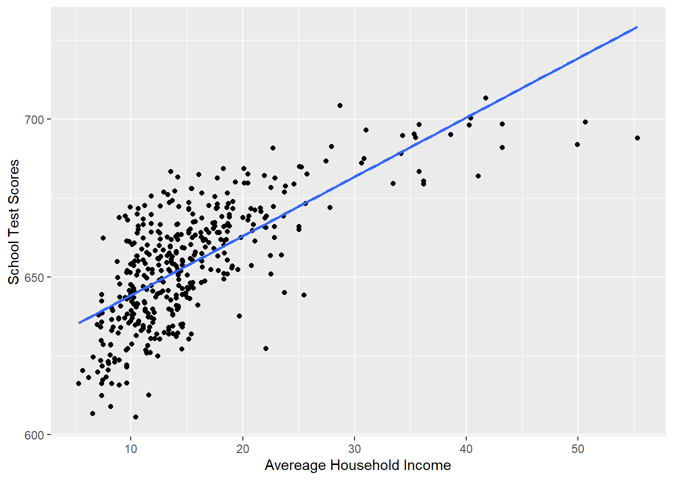
summary(lm(score ~ income, data=dat))
#>
#> Call:
#> lm(formula = score ~ income, data = dat)
#>
#> Residuals:
#>     Min      1Q  Median      3Q     Max
#> -39.574  -8.803   0.603   9.032  32.530
#>
#> Coefficients:
#>             Estimate Std. Error t value Pr(>|t|)
#> (Intercept) 625.3836     1.5324  408.11   <2e-16 ***
#> income        1.8785     0.0905   20.76   <2e-16 ***
#> ---
#> Signif. codes:
#> 0 '***' 0.001 '**' 0.01 '*' 0.05 '.' 0.1 ' ' 1
#>
#> Residual standard error: 13.39 on 418 degrees of freedom
#> Multiple R-squared:  0.5076, Adjusted R-squared:  0.5064
#> F-statistic: 430.8 on 1 and 418 DF,  p-value: < 2.2e-16
Just looking at this visually, does this line well represent this relationship? Not really, no.
The way we deal with this is adding polynomial terms to our regression. The easy way to think about polynomials is: it let’s the line curve.
To do this we modify the simple bivariate regression by adding an additional variable income squared:
\[ y = a + bx + e\\ y = a + b_1 x + b_2 x^2 + e \]
To implement this we can use the poly() function:
#YOU MUST USE THE RAW=T OPTION WHEN YOU USE THE POLY FUNCTION
#OR IT WILL NOT WORK

m <- lm(score ~ poly(income, 2, raw=T), data=dat )
summary(m)
#>
#> Call:
#> lm(formula = score ~ poly(income, 2, raw = T), data = dat)
#>
#> Residuals:
#>     Min      1Q  Median      3Q     Max
#> -44.416  -9.048   0.440   8.347  31.639
#>
#> Coefficients:
#>                            Estimate Std. Error t value
#> (Intercept)               607.30174    3.04622 199.362
#> poly(income, 2, raw = T)1   3.85099    0.30426  12.657
#> poly(income, 2, raw = T)2  -0.04231    0.00626  -6.758
#>                           Pr(>|t|)
#> (Intercept)                < 2e-16 ***
#> poly(income, 2, raw = T)1  < 2e-16 ***
#> poly(income, 2, raw = T)2 4.71e-11 ***
#> ---
#> Signif. codes:
#> 0 '***' 0.001 '**' 0.01 '*' 0.05 '.' 0.1 ' ' 1
#>
#> Residual standard error: 12.72 on 417 degrees of freedom
#> Multiple R-squared:  0.5562, Adjusted R-squared:  0.554
#> F-statistic: 261.3 on 2 and 417 DF,  p-value: < 2.2e-16

#This is equivalent to:

dat$income2  <- dat$income^2

m <- lm(score ~ income + income2, data=dat )
summary(m)
#>
#> Call:
#> lm(formula = score ~ income + income2, data = dat)
#>
#> Residuals:
#>     Min      1Q  Median      3Q     Max
#> -44.416  -9.048   0.440   8.347  31.639
#>
#> Coefficients:
#>              Estimate Std. Error t value Pr(>|t|)
#> (Intercept) 607.30174    3.04622 199.362  < 2e-16 ***
#> income        3.85099    0.30426  12.657  < 2e-16 ***
#> income2      -0.04231    0.00626  -6.758 4.71e-11 ***
#> ---
#> Signif. codes:
#> 0 '***' 0.001 '**' 0.01 '*' 0.05 '.' 0.1 ' ' 1
#>
#> Residual standard error: 12.72 on 417 degrees of freedom
#> Multiple R-squared:  0.5562, Adjusted R-squared:  0.554
#> F-statistic: 261.3 on 2 and 417 DF,  p-value: < 2.2e-16

#Plotting this relationship:
library(ggplot2)
p <- ggplot(dat, aes(x=income, y=score)) + geom_point() +
  labs(x="Avereage Household Income", y = "School Test Scores") +
  geom_smooth(method = lm, formula = y ~ poly(x, 2), se = FALSE)
p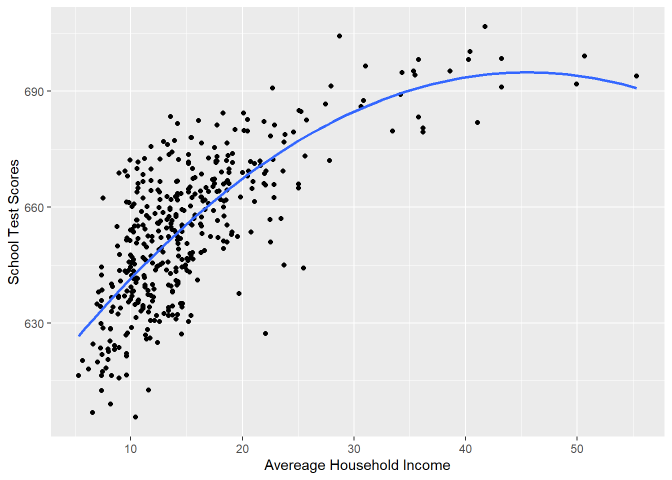
To get the effect of this variable we can take the first derivative using the power rule. A refresher on how the power rule works:
\[ \frac{\partial y}{\partial x}(X^k) =k*X^{k-1} \\ \frac{\partial y}{\partial x}(aX^k) =k*aX^{k-1} \\ \frac{\partial y}{\partial x}(a) =0 \\ \frac{\partial y}{\partial x}(Z) =0 \\ \]
Applying this to when we have polynomial term:
\[ \hat{y} = \hat{\alpha} + \hat{\beta_1}*x + \hat{\beta_2}*x^2 \\ \frac{\partial y}{\partial x} = \hat{\beta}_1 + 2*\hat{\beta_2}*x \]
So here, if we wanted to know the effect of income when income is at 20,30,50:
coef(m)
#>  (Intercept)       income      income2
#> 607.30174351   3.85099392  -0.04230845

coef(m)[2] + 2*coef(m)[3]*20
#>   income
#> 2.158656

#2.15
#and at 30
coef(m)[2] + 2*coef(m)[3]*30
#>   income
#> 1.312487

#and at 50
coef(m)[2] + 2*coef(m)[3]*50
#>     income
#> -0.3798508
The second violation of the functional form assumption is when our data comes from clusters but we are modeling it as if it is just a big random sample. In that case we want to explicitly model the clustered structure of the data. The canonical example of that is if you have students in a school: the relationship between the students home income and test scores will be derived, partly, from which classroom they are in. So to not violate this assumption we want to include a method that takes into account these clusters.
The example we saw in class was using the ACS data. Here the data comes from states. As such, the relationship between (for example) percent less than high school and the unemployment is determined, partly, by the state which a county is in. Another way to think about this is that the relationship within states is what we want to estimate because looking at this relationship between states introduces lots of bias. If we estimate between states part of our coefficient will be determined by state-level factors which lead to a higher percent of people with less than a high school education and higher unemployment.
To deal with this we can run a fixed-effects regression which gives an intercept to each state. See below for how we additionally have to adjust our standard errors for this clustered data.
names(acs)
#>  [1] "V1"                      "county.fips"
#>  [3] "county.name"             "state.full"
#>  [5] "state.abbr"              "state.alpha"
#>  [7] "state.icpsr"             "census.region"
#>  [9] "population"              "population.density"
#> [11] "percent.senior"          "percent.white"
#> [13] "percent.black"           "percent.asian"
#> [15] "percent.amerindian"      "percent.less.hs"
#> [17] "percent.college"         "unemployment.rate"
#> [19] "median.income"           "gini"
#> [21] "median.rent"             "percent.child.poverty"
#> [23] "percent.adult.poverty"   "percent.car.commute"
#> [25] "percent.transit.commute" "percent.bicycle.commute"
#> [27] "percent.walk.commute"    "average.commute.time"
#> [29] "percent.no.insurance"    "midwest"
#> [31] "northeast"               "south"
#> [33] "west"

#Standard
m <- lm(unemployment.rate ~ percent.less.hs, data=acs)
summary(m)
#>
#> Call:
#> lm(formula = unemployment.rate ~ percent.less.hs, data = acs)
#>
#> Residuals:
#>      Min       1Q   Median       3Q      Max
#> -16.3352  -1.5111  -0.1961   1.2056  21.3602
#>
#> Coefficients:
#>                 Estimate Std. Error t value Pr(>|t|)
#> (Intercept)     3.098618   0.106664   29.05   <2e-16 ***
#> percent.less.hs 0.199515   0.007192   27.74   <2e-16 ***
#> ---
#> Signif. codes:
#> 0 '***' 0.001 '**' 0.01 '*' 0.05 '.' 0.1 ' ' 1
#>
#> Residual standard error: 2.555 on 3139 degrees of freedom
#>   (1 observation deleted due to missingness)
#> Multiple R-squared:  0.1969, Adjusted R-squared:  0.1966
#> F-statistic: 769.6 on 1 and 3139 DF,  p-value: < 2.2e-16

#Fixed Effects
library(lfe)
#> Loading required package: Matrix
#> Warning: package 'Matrix' was built under R version 4.1.3
#>
#> Attaching package: 'lfe'
#> The following object is masked from 'package:lmtest':
#>
#>     waldtest
m.fe <- felm(unemployment.rate ~ percent.less.hs | state.abbr, data=acs)
summary(m.fe)
#>
#> Call:
#>    felm(formula = unemployment.rate ~ percent.less.hs | state.abbr,      data = acs)
#>
#> Residuals:
#>      Min       1Q   Median       3Q      Max
#> -13.1414  -1.3097  -0.1830   0.9995  20.7760
#>
#> Coefficients:
#>                 Estimate Std. Error t value Pr(>|t|)
#> percent.less.hs 0.160505   0.008225   19.52   <2e-16 ***
#> ---
#> Signif. codes:
#> 0 '***' 0.001 '**' 0.01 '*' 0.05 '.' 0.1 ' ' 1
#>
#> Residual standard error: 2.301 on 3089 degrees of freedom
#>   (1 observation deleted due to missingness)
#> Multiple R-squared(full model): 0.3591   Adjusted R-squared: 0.3486
#> Multiple R-squared(proj model): 0.1098   Adjusted R-squared: 0.09506
#> F-statistic(full model):33.94 on 51 and 3089 DF, p-value: < 2.2e-16
#> F-statistic(proj model): 380.8 on 1 and 3089 DF, p-value: < 2.2e-16

#Relationship somewhat attenuated.
The third violation of the functional form assumption is when we have to include an interaction term, which is dealt with in it’s own section, below.
15.8.3 3. No heteroskedasticity
Assumptions 3 & 4 deal with having incorrect standard errrors.
Assumption 3 says that, conditional on x, the squared error term must be equal to \(\sigma^2\). Less important here is what sigma squared is, and more important is that this is saying that the error must be constant across levels of X.
In short this assumption is violated if there is more variation in the dependent variable in some part of our independent variable. A pattern that may look like this:
#Heteroskedastic Errors
x <- runif(100, min=0, max=100)
y <- 2 + 3*x + rnorm(100, mean=0, sd=x*2)

plot(x,y)
abline(lm(y~x), col="firebrick" ,lwd=2)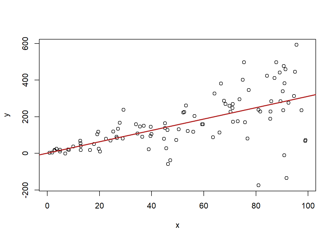
Here was a real-world example of heteroskedasticity:
dat$esl <- dat$english
plot( dat$esl, dat$math)
abline(lm(dat$math ~ dat$esl), col="firebrick", lwd=2)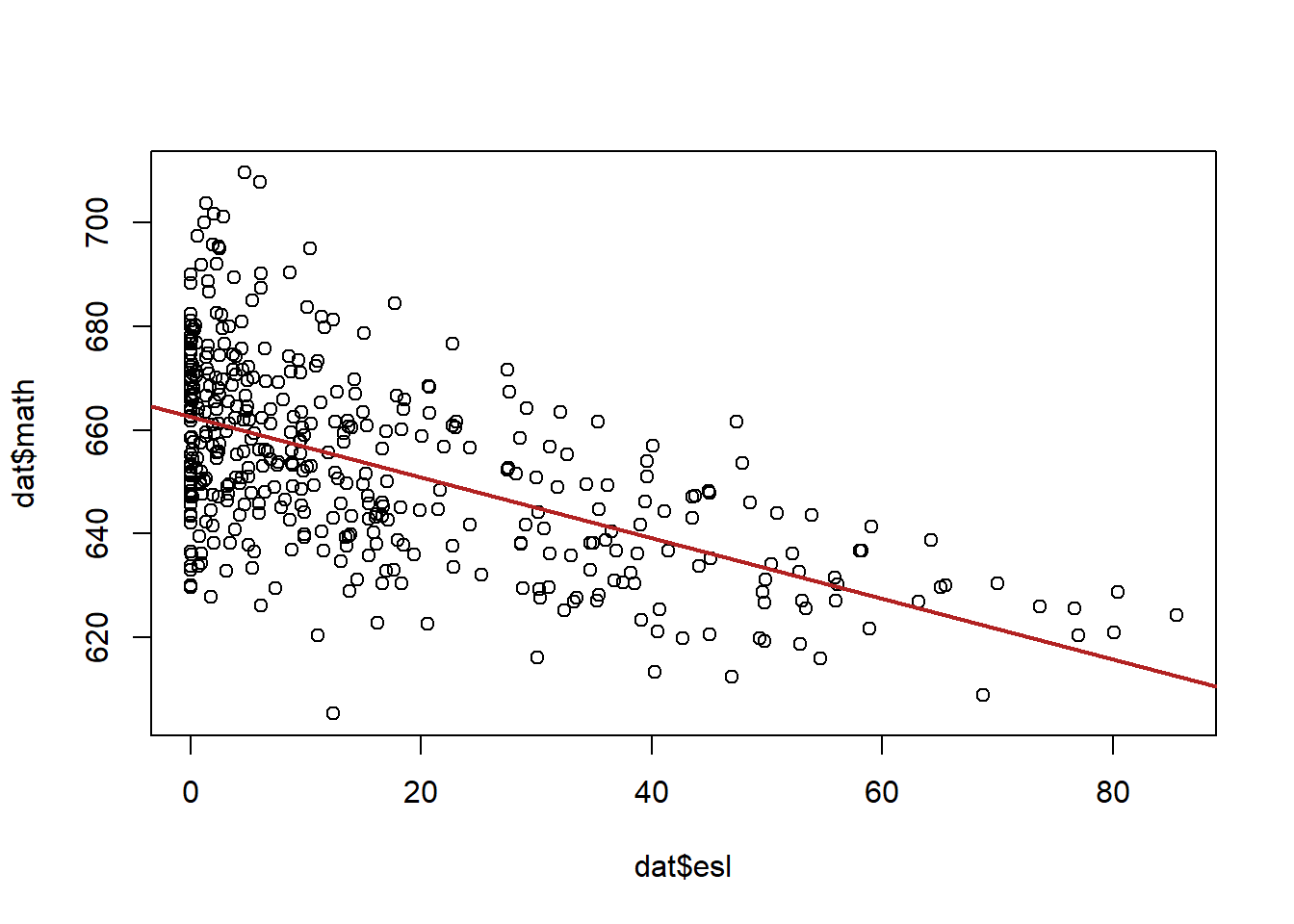
In general there seems to be a lot more variation in math scores when esl is lower, and less when esl is higher.
There is a specific test for heteroskedasticity beyond what we can see with our eyes:
library(lmtest)
m <- lm(math ~ esl, data=dat)
bptest(m)
#>
#>  studentized Breusch-Pagan test
#>
#> data:  m
#> BP = 12.084, df = 1, p-value = 0.0005085
This test will be statistically significant if heteroskedasticity is present. Here we reject the null hypothesis of homoskedasticity.
How can we fix this?
Well, one way to fix heteroskedasticity is to better model the reasons for higher variance in some cases.
We think that there is more unmodeled variance at the low end of esl. In other words schools without a lot of english as a second language children come from all different types of places. If we add variables that explain math scores among that group better heteroskedasticity will be reduced.
So, for example, if we add to our regression other variables which help us determine what sort of schools these are…
m <- lm(math ~ esl + lunch + calworks + income, data=dat)
summary(m)
#>
#> Call:
#> lm(formula = math ~ esl + lunch + calworks + income, data = dat)
#>
#> Residuals:
#>      Min       1Q   Median       3Q      Max
#> -30.8808  -6.6403  -0.0207   5.8995  30.0311
#>
#> Coefficients:
#>              Estimate Std. Error t value Pr(>|t|)
#> (Intercept) 660.25387    2.47171 267.124  < 2e-16 ***
#> esl          -0.14893    0.03831  -3.887 0.000118 ***
#> lunch        -0.32979    0.04215  -7.825 4.26e-14 ***
#> calworks     -0.11171    0.06657  -1.678 0.094090 .
#> income        0.76129    0.09542   7.979 1.46e-14 ***
#> ---
#> Signif. codes:
#> 0 '***' 0.001 '**' 0.01 '*' 0.05 '.' 0.1 ' ' 1
#>
#> Residual standard error: 9.928 on 415 degrees of freedom
#> Multiple R-squared:  0.7224, Adjusted R-squared:  0.7198
#> F-statistic:   270 on 4 and 415 DF,  p-value: < 2.2e-16
bptest(m)
#>
#>  studentized Breusch-Pagan test
#>
#> data:  m
#> BP = 7.4826, df = 4, p-value = 0.1125
We no longer have a heteroskedastic regression.
The other way to deal with heteroskedasticity is to employ Hubert-White (or simply “robust”) standard errors.
library(sandwich)
library(lmtest)
m <- lm(math ~ esl, data=dat)
robust.vcov <- vcovHC(m, type="HC1")
coeftest(m, vcov=robust.vcov)
#>
#> t test of coefficients:
#>
#>               Estimate Std. Error t value  Pr(>|t|)
#> (Intercept) 662.539315   1.046782 632.929 < 2.2e-16 ***
#> esl          -0.583245   0.033671 -17.322 < 2.2e-16 ***
#> ---
#> Signif. codes:
#> 0 '***' 0.001 '**' 0.01 '*' 0.05 '.' 0.1 ' ' 1
15.8.4 3. No autocorrelation
Assumption 4 talks about “auto-correlation”. This has the same problem of breaking the assumption that the errors of one data point are independent from others, but here it is because that points are related to one another in some un-modeled way. This is almost always due to time or to clusters.
Here is quarterly American GDP since the year 2000:
gdp <- import("https://github.com/marctrussler/IIS-Data/raw/main/GDP.csv")
gdp <- gdp[213:307,]

plot(gdp$DATE, gdp$GDP)
abline(lm(gdp$GDP ~ gdp$DATE), col="firebrick", lwd=2)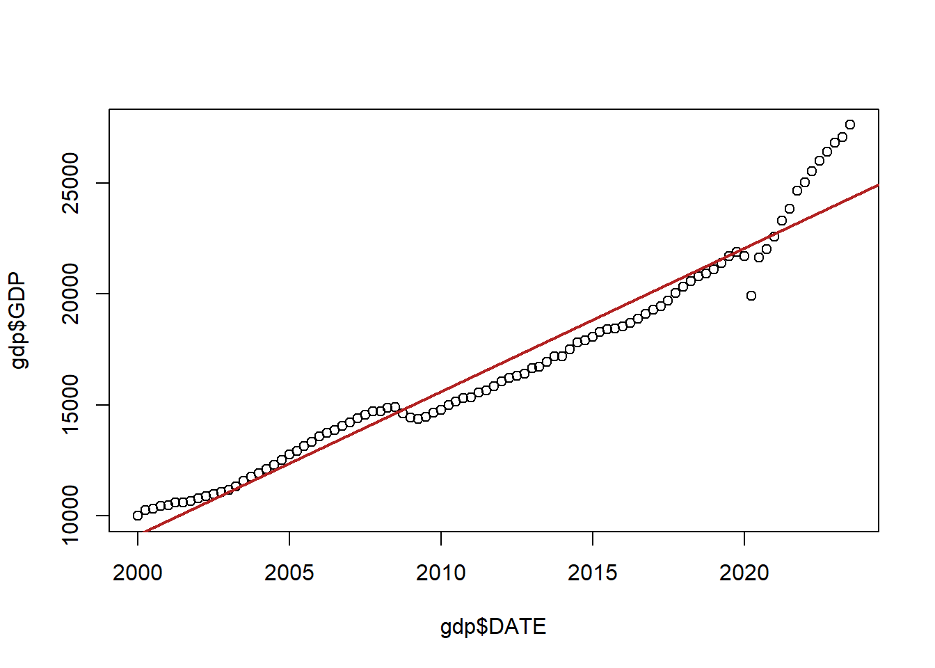
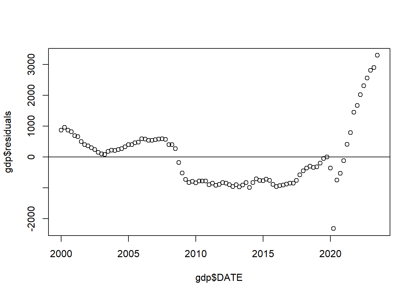
Now, ignoring the fact there that this red line doesn’t do a great job of fitting the data, the problem here is that the errors being made from point to point are not independent from one another.
Let’s look at the relationships between the date and the residuals from that regression:
For comparison, here is what this same plot looks like when things are fine (from the data we created abo:
x <- runif(100, min=0, max=100)
y <- 2 + 3*x + rnorm(100, mean=0, sd=15)
resid <- residuals(lm(y~x))
plot(x,resid)
abline(h=0)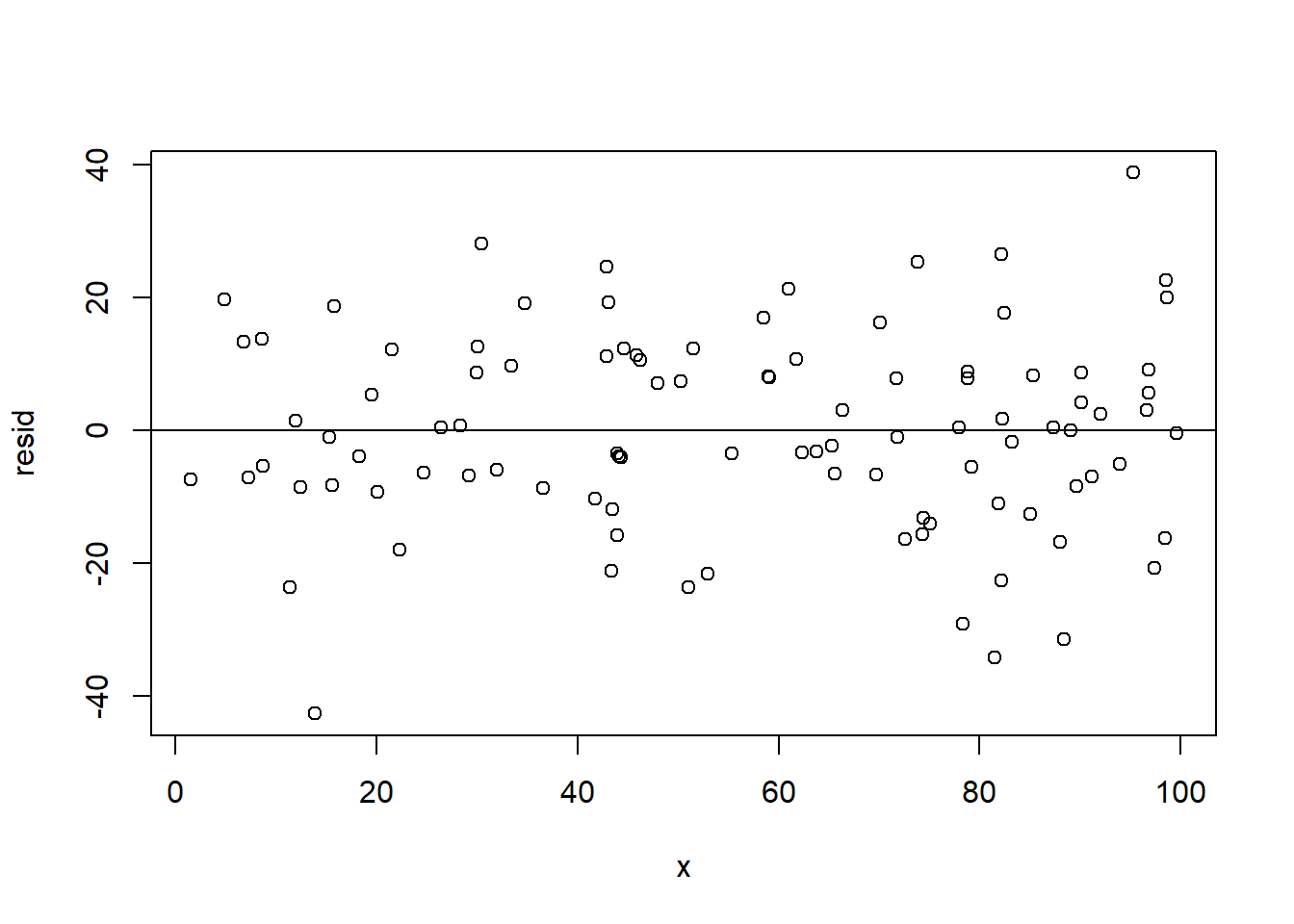
Here the error on one point doesn’t really tell you anything about its neighbors.
How do we deal with time-based autocorrelation? Run! It’s very hard to deal with and is the focus of full courses. For right now it’s enough to know that this sort of pattern runs counter to the assumption of OLS.
For cluster based-autocorrelation we want to use cluster robust standard errors.
Above, we used the sandwich package to generate heteroskedastic-robust standard errors. We can use the same package to generate clustered standard errors. In the vcovCL() function we can specify what variable our data are clustered on. Here it is state, so I’ve put that variable into the command. I’ve also included type="HC1" into this. This is actually the default so I didn’t have to put it in, but I wanted to point out that cluster standard errors are also heteroskedastic robust as well! A bonus!
m <- lm(median.income ~ percent.college, data=acs)
summary(m)
#>
#> Call:
#> lm(formula = median.income ~ percent.college, data = acs)
#>
#> Residuals:
#>    Min     1Q Median     3Q    Max
#> -37849  -6044   -623   5696  52223
#>
#> Coefficients:
#>                 Estimate Std. Error t value Pr(>|t|)
#> (Intercept)     29651.55     435.98   68.01   <2e-16 ***
#> percent.college  1016.55      18.52   54.90   <2e-16 ***
#> ---
#> Signif. codes:
#> 0 '***' 0.001 '**' 0.01 '*' 0.05 '.' 0.1 ' ' 1
#>
#> Residual standard error: 9789 on 3139 degrees of freedom
#>   (1 observation deleted due to missingness)
#> Multiple R-squared:  0.4899, Adjusted R-squared:  0.4897
#> F-statistic:  3014 on 1 and 3139 DF,  p-value: < 2.2e-16
library(sandwich)
cluster.vcov <- vcovCL(m, cluster= ~ state.abbr, type="HC1")
cluster.vcov2 <- vcovCL(m, cluster= ~ state.abbr)

#Compare to original var-covar matrix
vcov(m)
#>                 (Intercept) percent.college
#> (Intercept)      190078.663      -7396.2115
#> percent.college   -7396.212        342.8198
#New hypothesis test
coeftest(m, vcov = cluster.vcov )
#>
#> t test of coefficients:
#>
#>                  Estimate Std. Error t value  Pr(>|t|)
#> (Intercept)     29651.551   1337.982  22.161 < 2.2e-16 ***
#> percent.college  1016.547     55.331  18.372 < 2.2e-16 ***
#> ---
#> Signif. codes:
#> 0 '***' 0.001 '**' 0.01 '*' 0.05 '.' 0.1 ' ' 1
Finally, tieing this in with GM2, if we choose to explicitly model the clusters in our dataset, we also have to use cluster-robust standard errors. The felm command will do this for you:
#Normal SE
m.fe <- felm(unemployment.rate ~ percent.less.hs | state.abbr, data=acs)
summary(m.fe)
#>
#> Call:
#>    felm(formula = unemployment.rate ~ percent.less.hs | state.abbr,      data = acs)
#>
#> Residuals:
#>      Min       1Q   Median       3Q      Max
#> -13.1414  -1.3097  -0.1830   0.9995  20.7760
#>
#> Coefficients:
#>                 Estimate Std. Error t value Pr(>|t|)
#> percent.less.hs 0.160505   0.008225   19.52   <2e-16 ***
#> ---
#> Signif. codes:
#> 0 '***' 0.001 '**' 0.01 '*' 0.05 '.' 0.1 ' ' 1
#>
#> Residual standard error: 2.301 on 3089 degrees of freedom
#>   (1 observation deleted due to missingness)
#> Multiple R-squared(full model): 0.3591   Adjusted R-squared: 0.3486
#> Multiple R-squared(proj model): 0.1098   Adjusted R-squared: 0.09506
#> F-statistic(full model):33.94 on 51 and 3089 DF, p-value: < 2.2e-16
#> F-statistic(proj model): 380.8 on 1 and 3089 DF, p-value: < 2.2e-16
#Cluster-Robust SE
m.fe.clu <- felm(unemployment.rate ~ percent.less.hs | state.abbr| 0 | state.abbr, data=acs)
summary(m.fe.clu)
#>
#> Call:
#>    felm(formula = unemployment.rate ~ percent.less.hs | state.abbr |      0 | state.abbr, data = acs)
#>
#> Residuals:
#>      Min       1Q   Median       3Q      Max
#> -13.1414  -1.3097  -0.1830   0.9995  20.7760
#>
#> Coefficients:
#>                 Estimate Cluster s.e. t value Pr(>|t|)
#> percent.less.hs   0.1605       0.0289   5.553 1.07e-06 ***
#> ---
#> Signif. codes:
#> 0 '***' 0.001 '**' 0.01 '*' 0.05 '.' 0.1 ' ' 1
#>
#> Residual standard error: 2.301 on 3089 degrees of freedom
#>   (1 observation deleted due to missingness)
#> Multiple R-squared(full model): 0.3591   Adjusted R-squared: 0.3486
#> Multiple R-squared(proj model): 0.1098   Adjusted R-squared: 0.09506
#> F-statistic(full model, *iid*):33.94 on 51 and 3089 DF, p-value: < 2.2e-16
#> F-statistic(proj model): 30.84 on 1 and 50 DF, p-value: 1.073e-06
15.8.5 5. Causality
The last Gauss-Markov assumption is that there are no omitted variables which impact both x and y. This is often thought of as the “bonus” assumption as it is not strictly necessary to have an unbiased estimator. We didn’t talk much about causality in this class beyond omitted variables. It’s a really big subject!
15.9 Regression Interaction and Prediction
15.9.1 Interaction
We can think of interaction as another potential violation to GM2. In this case the true data generating process is one where the effect of one variable depends on another. Indeed, if it’s helpful we can think of polynomial regression as a subset of interactive regression where the effect of a variablt depends on itself.
The most helpful way to think about interaction is via the regression equation. An interactive regression looks like this:
\[ \hat{Y} = \hat{\alpha} + \hat{\beta_1}X + \hat{\beta_2}Z + \hat{\beta_3}X*Z \]
Once we use the power rule to take the first derivative of this equation with respect to both X and Z:
\[ \frac{\partial \hat{Y}}{\partial X} = \hat{\beta_1} + \hat{\beta_3}Z \]
This equation gives us what the effect of X on Y is. The things that are true from this are: (1) \(\beta_1\) represents the effect of X on Y when Z is zero; (2) \(\beta_3\) represents how a 1-unit change in Z alters the relationship between X and Y.
Critically, interaction is completely symmetrical such that:
\[ \frac{\partial \hat{y}}{\partial Z} = \hat{\beta_1} + \hat{\beta_3}X \]
To give an example, we can think about how the the relationship between median income and income inequality is altered by the percent of a county who is white:
library(rio)
library(stargazer)
#>
#> Please cite as:
#>  Hlavac, Marek (2018). stargazer: Well-Formatted Regression and Summary Statistics Tables.
#>  R package version 5.2.2. https://CRAN.R-project.org/package=stargazer
acs <- import("https://github.com/marctrussler/IIS-Data/raw/main/ACSCountyData.csv")

acs$median.income <- acs$median.income/1000
acs$gini <- acs$gini*100

m4 <- lm(gini ~ median.income*percent.white, data=acs)
summary(m4)
#>
#> Call:
#> lm(formula = gini ~ median.income * percent.white, data = acs)
#>
#> Residuals:
#>      Min       1Q   Median       3Q      Max
#> -14.7470  -1.9791  -0.2637   1.8651  17.0992
#>
#> Coefficients:
#>                               Estimate Std. Error t value
#> (Intercept)                 52.5755392  0.8567078  61.369
#> median.income               -0.0365980  0.0178957  -2.045
#> percent.white               -0.0386569  0.0109061  -3.545
#> median.income:percent.white -0.0006808  0.0002248  -3.029
#>                             Pr(>|t|)
#> (Intercept)                  < 2e-16 ***
#> median.income               0.040932 *
#> percent.white               0.000399 ***
#> median.income:percent.white 0.002476 **
#> ---
#> Signif. codes:
#> 0 '***' 0.001 '**' 0.01 '*' 0.05 '.' 0.1 ' ' 1
#>
#> Residual standard error: 3.166 on 3137 degrees of freedom
#>   (1 observation deleted due to missingness)
#> Multiple R-squared:  0.249,  Adjusted R-squared:  0.2483
#> F-statistic: 346.7 on 3 and 3137 DF,  p-value: < 2.2e-16
We can use the full regression equation and put in numbers for median income and percent white to look at how the relationship looks at different levels:
median.income <- seq(0,150,.01)

pred0 <- coef(m4)["(Intercept)"] +
  coef(m4)["median.income"]*median.income +
  coef(m4)["percent.white"]*0 +
  coef(m4)["median.income:percent.white"]*0*median.income
pred25 <- coef(m4)["(Intercept)"] +
  coef(m4)["median.income"]*median.income +
  coef(m4)["percent.white"]*25 +
  coef(m4)["median.income:percent.white"]*25*median.income
pred50 <- coef(m4)["(Intercept)"] +
  coef(m4)["median.income"]*median.income +
  coef(m4)["percent.white"]*50 +
  coef(m4)["median.income:percent.white"]*50*median.income
pred75 <- coef(m4)["(Intercept)"] +
  coef(m4)["median.income"]*median.income +
  coef(m4)["percent.white"]*75 +
  coef(m4)["median.income:percent.white"]*75*median.income
pred100 <- coef(m4)["(Intercept)"] +
  coef(m4)["median.income"]*median.income +
  coef(m4)["percent.white"]*100 +
  coef(m4)["median.income:percent.white"]*100*median.income

library(RColorBrewer)
#> Warning: package 'RColorBrewer' was built under R version
#> 4.1.3

cols <- brewer.pal(7, "Set2")

plot(acs$median.income, acs$gini, col="gray80")
points(median.income, pred0,lwd=2, type="l", col=cols[1])
points(median.income, pred25,lwd=2, type="l", col=cols[2])
points(median.income, pred50,lwd=2, type="l",  col=cols[3])
points(median.income, pred75,lwd=2, type="l",  col=cols[4])
points(median.income, pred100,lwd=2, type="l",  col=cols[5])
legend("topleft", c("0% White",
                    "25% White",
                    "50% White",
                    "75% White",
                    "100% White"),
       lty=rep(1,6), col=cols)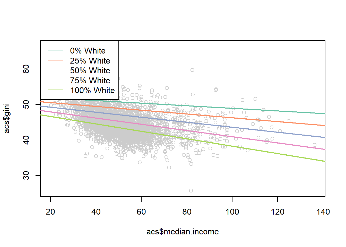
Alternatively we can just look at the marginal effect of one of the variables across the levels of the other:
#Manually
percent.white <- seq(0,100,.01)

margin <- coef(m4)["median.income"] + coef(m4)["median.income:percent.white"]*percent.white

plot(percent.white, margin, type="l", ylim=c(-0.15,0))
abline(h=0, lty=2)
rug(acs$percent.white)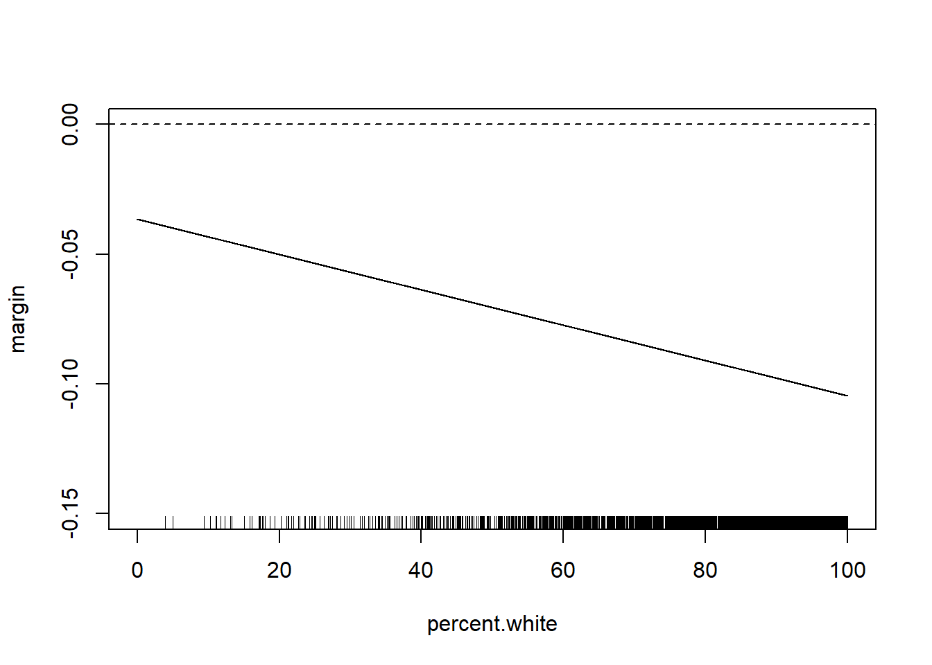
#Via the Margins Package
library(margins)
#> Warning: package 'margins' was built under R version 4.1.3
cplot(m4, x="median.income",dx="percent.white", what="effect")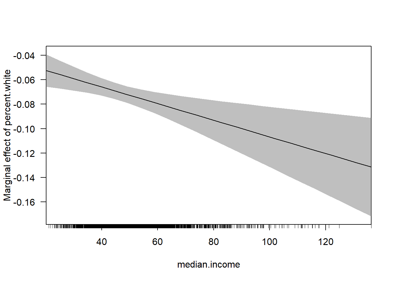
cplot(m4, dx="median.income",x="percent.white", what="effect")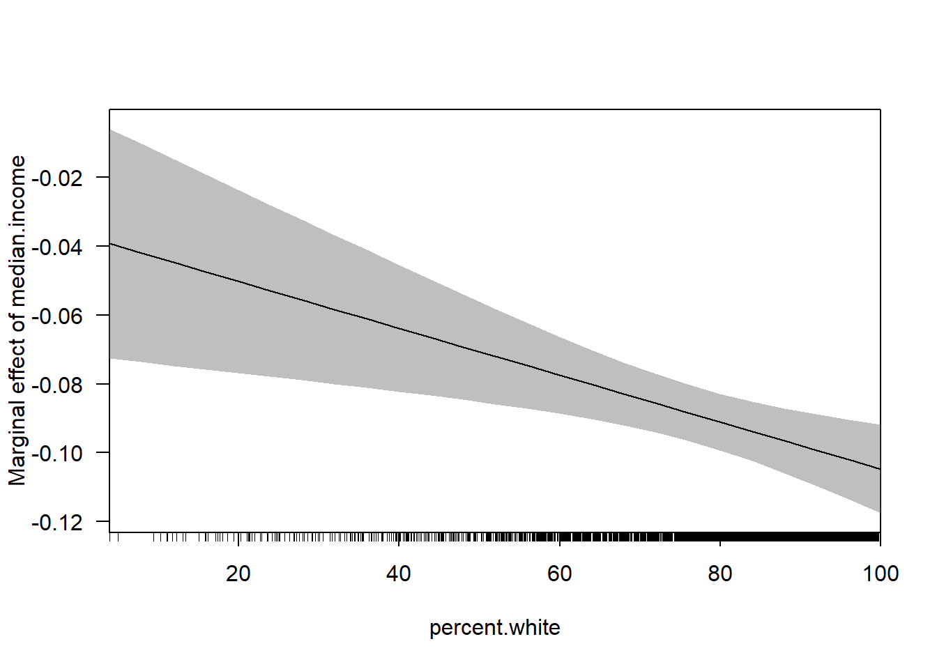
15.9.2 Prediction
Regression with prediction is relatively straightforward. If we have a regression equation where we have estimated the betas and alpha, we can put whatever we want in for the variables and the equation will spit out a predicted value of y. It’s therefore quite easy to form predictions.
We looked at this through the lens of making likely voter predictions.
We have previous year data where we know who voted and who didn’t, so we can build a model of voting:
table(cces$vote.intent)
#>
#> Already voted         Maybe            No           Yes
#>         16563         23491         15139        130199
cces$vote.intent <- factor(cces$vote.intent)
cces$vote.intent <- relevel(cces$vote.intent, ref="No")

cces.training <- cces[cces$year %in% c(2016,2018),]
cces.test <- cces[cces$year==2020,]

m2 <- lm(vv.turnout ~  vote.intent +prim.turnout + educ:white, data=cces.training)
summary(m2)
#>
#> Call:
#> lm(formula = vv.turnout ~ vote.intent + prim.turnout + educ:white,
#>     data = cces.training)
#>
#> Residuals:
#>      Min       1Q   Median       3Q      Max
#> -1.04559 -0.46192  0.00272  0.43795  1.01201
#>
#> Coefficients: (1 not defined because of singularities)
#>                                 Estimate Std. Error t value
#> (Intercept)                     0.110132   0.004586  24.014
#> vote.intentAlready voted        0.500227   0.007369  67.882
#> vote.intentMaybe                0.163265   0.004999  32.657
#> vote.intentYes                  0.473932   0.004296 110.316
#> prim.turnout                    0.435233   0.002883 150.948
#> educcollege:whitenonwhite      -0.116630   0.005081 -22.953
#> educHS or less:whitenonwhite   -0.122144   0.005088 -24.009
#> educpostgrad:whitenonwhite     -0.087024   0.007057 -12.332
#> educsome college:whitenonwhite -0.080891   0.004382 -18.459
#> educcollege:whitewhite         -0.022178   0.003726  -5.953
#> educHS or less:whitewhite      -0.033830   0.003439  -9.838
#> educpostgrad:whitewhite        -0.022014   0.004334  -5.079
#> educsome college:whitewhite           NA         NA      NA
#>                                Pr(>|t|)
#> (Intercept)                     < 2e-16 ***
#> vote.intentAlready voted        < 2e-16 ***
#> vote.intentMaybe                < 2e-16 ***
#> vote.intentYes                  < 2e-16 ***
#> prim.turnout                    < 2e-16 ***
#> educcollege:whitenonwhite       < 2e-16 ***
#> educHS or less:whitenonwhite    < 2e-16 ***
#> educpostgrad:whitenonwhite      < 2e-16 ***
#> educsome college:whitenonwhite  < 2e-16 ***
#> educcollege:whitewhite         2.64e-09 ***
#> educHS or less:whitewhite       < 2e-16 ***
#> educpostgrad:whitewhite        3.79e-07 ***
#> educsome college:whitewhite          NA
#> ---
#> Signif. codes:
#> 0 '***' 0.001 '**' 0.01 '*' 0.05 '.' 0.1 ' ' 1
#>
#> Residual standard error: 0.4087 on 124436 degrees of freedom
#>   (152 observations deleted due to missingness)
#> Multiple R-squared:  0.3225, Adjusted R-squared:  0.3225
#> F-statistic:  5386 on 11 and 124436 DF,  p-value: < 2.2e-16
If we have a dataset (here data from the same survey from a more recent year) that has the same variables in it, we can use the estiamted coefficients from our “training” model to predict among the “test” data the probaility of voting, or not:
cces.test$predict2 <- predict(m2, newdata=cces.test)
#> Warning in predict.lm(m2, newdata = cces.test): prediction
#> from a rank-deficient fit may be misleading
head(cces.test)
#>            V1 year vv.turnout         educ white female
#> 124601 124601 2020          1 some college white      0
#> 124602 124602 2020          0     postgrad white      1
#> 124603 124603 2020          0      college white      1
#> 124604 124604 2020          1      college white      1
#> 124605 124605 2020          0      college white      0
#> 124606 124606 2020          1 some college white      0
#>        agegrp   vote.intent pid3 prim.turnout   predict2
#> 124601  50-64 Already voted    2            1 1.04559165
#> 124602  65-74            No    1            0 0.08811756
#> 124603  65-74           Yes    3            0 0.56188595
#> 124604  50-64           Yes    1            1 0.99711855
#> 124605  50-64           Yes    3            0 0.56188595
#> 124606  50-64           Yes    2            0 0.58406435
table(cces.test$predict2)
#>
#>  -0.0120123927780443 -0.00649795413115195
#>                  762                  195
#>   0.0231077649957248   0.0292410289131809
#>                  128                  457
#>   0.0763023968785974   0.0879535214186681
#>                 1825                  174
#>   0.0881175633502864    0.110131921968922
#>                   70                  660
#>    0.151252369038693    0.156766807685586
#>                 1034                  257
#>    0.186372526812462    0.192505790729918
#>                  106                  693
#>    0.239567158695335    0.251218283235406
#>                 1897                  363
#>    0.251382325167024     0.27339668378566
#>                  129                  991
#>    0.423220206162353    0.428734644809246
#>                   17                    1
#>    0.461920033301611    0.464473627853578
#>                 1777                   10
#>    0.467434471948504     0.48821473327331
#>                 1455                  386
#>    0.493729171920202     0.49704019107538
#>                  335                  593
#>    0.503173454992836    0.511534995818995
#>                 2362                   32
#>    0.523186120359066    0.523334891047079
#>                   10                  183
#>    0.523350162290684    0.529468154964535
#>                    2                  599
#>     0.54536452090932    0.550234822958253
#>                   18                 4642
#>    0.561885947498324    0.562049989429942
#>                 3316                 1635
#>    0.576529522929951    0.584064348048578
#>                  996                 4639
#>    0.586484967979091    0.588180647470022
#>                   27                  769
#>     0.58834468940164    0.591999406625983
#>                  480                   20
#>    0.610359048020276     0.62160512575286
#>                 1033                    5
#>    0.627738389670316    0.674799757635732
#>                   48                   86
#>    0.686450882175803    0.686614924107421
#>                   59                   17
#>    0.708629282726057    0.897152632242009
#>                   65                  554
#>    0.902667070888901    0.923447332213707
#>                 1121                  239
#>      0.9289617708606    0.932272790015778
#>                  430                  674
#>    0.938406053933234    0.958567489987476
#>                 1487                  329
#>    0.964700753904932     0.98546742189865
#>                  578                 3216
#>    0.997118546438721    0.997282588370339
#>                 4019                 2739
#>     1.01176212187035     1.01929694698898
#>                 1087                 4561
#>     1.02341324641042     1.02357728834204
#>                 1617                 1283
#>     1.04559164696067
#>                 1652
We can classify each person as a likely voter or not if there probability of voting is above or below 50%. From that we can determine how good of a job this model does in predicting 2020 voters. We can look to see the proportion of voters who are incorrectly classified. IE, how many are predicted to vote but don’t, and how many are predicted not to vote but do?
#Classification Error
mean((cces.test$predict2>.5 & cces.test$vv.turnout==0) | (cces.test$predict2<.5 & cces.test$vv.turnout==1),na.rm=T)
#> [1] 0.2115221