2 R Crash Course
2.1 Basics of R
This course is designed for people who already have a basic familiarity with R. This chapter serves as a refresher on basic concepts, and highlights some specific use cases that will be important for the way we will use R in this course.
You should have available the file RCrashCourse.R. If you load that file it will load all of the R code in this chapter in a script into R.
As a reminder: Information in your script window are codes that can be run, but they won’t be run until we send them to the console by either highlighting them and pressing run, or by using ctrl+enter (cmd+enter on Mac).
To start with, we can run some basic commands to remind ourselves that R can work simply as a calculator:
2.2 Objects
But that’s not what is interesting about R.
R becomes helpful because we can create and save objects.
You can think about objects as shortcuts to information. When you define an object R literally thinks as that object as the thing you defined it as.
result <- 5+3

#See that result is now in the "Environment" tab

#Now run that object:
result
#> [1] 8
To be clear there is nothing special about the word “result” here. We could have called this anything:
batman <- 5+3

batman
#> [1] 8
What happens if you try to overwrite a value?
batman <- "Bruce Wayne"

batman
#> [1] "Bruce Wayne"
It’s gone forever!
That seems like it might be a huge problem, but we actually don’t care. Everything that we have done up to this point is recorded in our script. The creation of “result”, the definition of “batman”. If we save nothing but our script, close R and open it again we can just run those same commands and end up in the same spot. This is a key benefit of working in R over something like excel. We don’t need to worry at all about saving a new version of our data with changes we made, all we need to do is to have stable inputs and a road map (a script) to get to where we were last time.
Some other small things with R:
Nearly everything is case sensitive.
#What happens if you uncommend and try to run this:
#Batman
Objects have different classes. batman is a character object (words/letters) and result is a numeric object.
We define character ojects using question marks. But note that even if we enter the number 8 as a character we cannot perform math on it:
Result <- "8"
#You can perform arithmetic functions on an object


result/8
#> [1] 1

#.... But not when that object is a character. Uncomment and try to run the following:

#Result/8
2.3 Functions
We have now defined several ojects in R. The next thing that we can do is apply a function to an object. A function is simply a preset operation that can apply to an object (if applying that function to that object is appropriate).
For example if we want to know the square root of result we could use math:
result^0.5
#> [1] 2.828427
But R has a built in function that allows us to do the same thing
sqrt(result)
#> [1] 2.828427
Again if we try to run a function on an object for which it doesn’t make sense:
#Uncomment this
#sqrt(batman)

#But we could do...
nchar(batman)
#> [1] 11
A key function is class(), which will let you know what things are:
2.4 Vectors
So far this doesn’t seem very interesting, and doesn’t look much like excel. What about data, where we have multiple observations of a variable.
The concept of vectors in R are where we start getting to that information.
Let’s say we know have this data on the world population in millions every decade:
| Year | World Pop (Millions) |
|---|---|
| 1950 | 2525 |
| 1960 | 3026 |
| 1970 | 3691 |
| 1980 | 4449 |
| 1990 | 5320 |
| 2000 | 6127 |
| 2010 | 6916 |
We can make use of that by entering those numbers as a vector. To do that we can use the concatenate function c().
world.pop<- c(2525,3026,3691,4449,5320,6127,6916)
world.pop
#> [1] 2525 3026 3691 4449 5320 6127 6916
The concatenate function can also combine multiple objects:
pop1 <- c(2525,3026,3691)
pop2 <- c(4449,5320,6127,6916)

world.pop <- c(pop1, pop2)
world.pop
#> [1] 2525 3026 3691 4449 5320 6127 6916
One of the most important functionalities in R is the use of square brackets. Square brackets allow us to select or isolate certain entries in a vector (and eventually, in matrices).
World pop has 7 entried (we can see this in the environment). If we wanted to pull out cetain entries:
world.pop[6]
#> [1] 6127
world.pop[2]
#> [1] 3026
But if we try to find out what the 8th entry in world pop is:
world.pop[8]
#> [1] NA
It returns an NA because there is no 8th entry.
What if we want more than one value. For example what if we want to return the 2nd and 5th values? One thing we can’t do (and R will almost immediately tell us):
#Uncomment and try to run this code:
#world.pop[2 5]
What about if we try to use a comma?
#Uncomment and try to run this code:
#world.pop[2,5]
This also doesn’t work, and R tells me this is the “incorrect number of dimensions”. Remember that error because it’s going to make a lot more sense very shortly.
What we need to do is to say to R: here is a list of the entries that we want. What have we seen that gives us a list of numbers? That’s right, concatenate!
world.pop[c(2,5)]
#> [1] 3026 5320
What if we want the 2,3,4,5 entries? Well we just learned that we can do:
world.pop[c(2,3,4,5)]
#> [1] 3026 3691 4449 5320
That works fine, but what if we had a much larger vector and wanted to grab, say, 100, values? We are not going to type all of those in. Instead we can use the functionality in R where if we put a colon between two integers it will give us the sequence from the first to the second integer.
2:5
#> [1] 2 3 4 5
world.pop[2:5]
#> [1] 3026 3691 4449 5320
Notice that just running 2:5 returned a vector of 2 3 4 5. There was no need to do c(2:5).
What if we want to do the opposite: produce a vector without a particular number. We can use the same principles but put a minus sign in front of the numbers in the square bracket:
#Using a minus sign will print the vector without whatever you specified

world.pop[-3]
#> [1] 2525 3026 4449 5320 6127 6916
world.pop[-c(2,5)]
#> [1] 2525 3691 4449 6127 6916
world.pop[c(-2,-5)]
#> [1] 2525 3691 4449 6127 6916
world.pop[-2:-5]
#> [1] 2525 6127 6916

#Why not:
#-2:5
#?
Because this is a numeric vector we can apply an arithmetic operation to the whole thing, and it will be applied to each value individually
world.pop*1000000
#> [1] 2.525e+09 3.026e+09 3.691e+09 4.449e+09 5.320e+09
#> [6] 6.127e+09 6.916e+09
What if we wanted to create a new object, that was the world population in each year as a proportion of the world population in 1950? We can just use basic arithmetic.
world.pop/world.pop[1]
#> [1] 1.000000 1.198416 1.461782 1.761980 2.106931 2.426535
#> [7] 2.739010
#Save it as a new object
pop.rate <- world.pop/world.pop[1]
pop.rate
#> [1] 1.000000 1.198416 1.461782 1.761980 2.106931 2.426535
#> [7] 2.739010
2.5 Simple Matrices
Now we have two vectors that describe information for the decades 1950 to 2010. We know that they are the same length. Right now R is just treating them as two seperate things but we know we can start thinking of this as sort of a table of information.
Let’s learn how to make R think about this as one thing.
First let’s create a vector of years so we know what each observation represents:
year <- c(1950,1960,1970,1980,1990,2000,2010)Now we want to put these three vectors of 7 items together into a table
year
#> [1] 1950 1960 1970 1980 1990 2000 2010
world.pop
#> [1] 2525 3026 3691 4449 5320 6127 6916
pop.rate
#> [1] 1.000000 1.198416 1.461782 1.761980 2.106931 2.426535
#> [7] 2.739010
To do this we can use the cbind() function, which is short for “column-bind”. While the c() function takes individual items and makes them a vector, cbind() takes vectors and turns them into a small table, which we will call a simple matrix.
cbind(year,world.pop,pop.rate)
#>      year world.pop pop.rate
#> [1,] 1950      2525 1.000000
#> [2,] 1960      3026 1.198416
#> [3,] 1970      3691 1.461782
#> [4,] 1980      4449 1.761980
#> [5,] 1990      5320 2.106931
#> [6,] 2000      6127 2.426535
#> [7,] 2010      6916 2.739010
We can, of course, save this:
population.table <- cbind(year,world.pop,pop.rate)

population.table
#>      year world.pop pop.rate
#> [1,] 1950      2525 1.000000
#> [2,] 1960      3026 1.198416
#> [3,] 1970      3691 1.461782
#> [4,] 1980      4449 1.761980
#> [5,] 1990      5320 2.106931
#> [6,] 2000      6127 2.426535
#> [7,] 2010      6916 2.739010
Now we have something the looks like excel!
Let’s practice adding another variable. What if we additionally have co2 emissions for each decade as well?
| Year | World Pop (Millions) | co2 Emissions |
|---|---|---|
| 1950 | 2525 | 6.00 |
| 1960 | 3026 | 9.33 |
| 1970 | 3691 | 14.83 |
| 1980 | 4449 | 19.37 |
| 1990 | 5320 | 22.70 |
| 2000 | 6127 | 25.12 |
| 2010 | 6916 | 33.13 |
emissions <- c(6,9.33,14.83,19.37,22.7,25.12,33.13)There are two ways to add this information.
We could build the table again from scratch, this time with emissions:
population.table.new <- cbind(year,world.pop,pop.rate, emissions)Or we can just cbind() emissions to our existing table:
population.table <- cbind(population.table, emissions)Now we have a small table. How can we access the information in this table?
The functionality of square brackets extends when we have a simple matrix like this, using the convention X[row,column]. We can use the comma to give information about the rows and columns we wish to access in the matrix.
For example
#To see the 1st entry in the 3rd row:


population.table[3,1]
#> year
#> 1970

#Or the 3rd entry in the 1st row

population.table[1,3]
#> pop.rate
#>        1
This should make it clear why we couldn’t use commas above on a 1-dimensional vector to get multiple items and why we had to use c().
Importantly, we can also pull out entire rows or columns by leaving either the row or column information blank:
#The first row
population.table[1, ]
#>      year world.pop  pop.rate emissions
#>      1950      2525         1         6
#The second column
population.table[ ,2]
#> [1] 2525 3026 3691 4449 5320 6127 6916
And appropriately, we can run functions on individual columns:
#We can run functions just on individual columns


mean(population.table[,2])
#> [1] 4579.143

min(population.table[,2])
#> [1] 2525

max(population.table[,2])
#> [1] 6916

range(population.table[,2])
#> [1] 2525 6916

sum(population.table[,2])
#> [1] 32054
Note that there is a special value in R NA which represents missing data. Having an NA in a column can break these functions
Let’s say we didn’t know the world population in 1980. That would mean the world.pop and pop.rate would be missing data.
population.table
#>      year world.pop pop.rate emissions
#> [1,] 1950      2525 1.000000      6.00
#> [2,] 1960      3026 1.198416      9.33
#> [3,] 1970      3691 1.461782     14.83
#> [4,] 1980      4449 1.761980     19.37
#> [5,] 1990      5320 2.106931     22.70
#> [6,] 2000      6127 2.426535     25.12
#> [7,] 2010      6916 2.739010     33.13

population.table[4,2:3]
#>  world.pop   pop.rate
#> 4449.00000    1.76198

population.table[4,2:3] <- NA

population.table
#>      year world.pop pop.rate emissions
#> [1,] 1950      2525 1.000000      6.00
#> [2,] 1960      3026 1.198416      9.33
#> [3,] 1970      3691 1.461782     14.83
#> [4,] 1980        NA       NA     19.37
#> [5,] 1990      5320 2.106931     22.70
#> [6,] 2000      6127 2.426535     25.12
#> [7,] 2010      6916 2.739010     33.13
What happens now if we take the mean of the second column (the world population)?
mean(population.table[,2])
#> [1] NA
This breaks R! It is very literal. What’s the average of 2,3, and something that is not a number. I don’t know!
Critically, there is an “option” for the mean function na.rm=T that will tell it to ignore NA and give you the mean of the remaining numbers.
#But we can just tell R to leave out any NAs and calcualte the mean:
mean(population.table[,2],na.rm=T)
#> [1] 4600.833
This isn’t just for the mean() function. Lots of functions, like sum(), max() or range() will also require na.rm=T.
#We can also use the locations if we want to make corrections if need be
#What if we want to go back in and replace those missing values (4449 for population,
#1.76198 for pop.rate). How might we do that?


population.table[4,2:3] <- c(4449,1.76198)
population.table
#>      year world.pop pop.rate emissions
#> [1,] 1950      2525 1.000000      6.00
#> [2,] 1960      3026 1.198416      9.33
#> [3,] 1970      3691 1.461782     14.83
#> [4,] 1980      4449 1.761980     19.37
#> [5,] 1990      5320 2.106931     22.70
#> [6,] 2000      6127 2.426535     25.12
#> [7,] 2010      6916 2.739010     33.13
The above problems with NAs has also introduced the concept of options to a function. We can see that we have added the option na.rm=T into the function by using a comma. Functions will often have many options. You can seel all the options and the default options by accessing the help file.
For example: what if we want to know the correlation betwen world population and emissions?
#?corWe see in the help file that correlation takes two vectors, an x and y vector. There is an option that tells it what observations to use (how it deals with missing values), and which type of correlation to use.
So in running a correlation we can do:
cor(population.table[,2], population.table[,4], use="everything",
    method="pearson")
#> [1] 0.9889095
But the help file will also show you what the defaults are, so if you leave out the options we will get the same thing:
cor(population.table[,2], population.table[,4])
#> [1] 0.9889095
2.6 Simple scatterplots
We now have enough data to make some simple scatterplots.
What if we want to graph a scatter plot with year on x axis, and world pop on the y axis
The basic plot() command is what we will use for scatterplots:
#?plotWhen we run a scatterplot, the first two “options” in the command will be the values of our points with the first being the horizontal values, and the second being the vertical values
plot(population.table[,1], population.table[,2])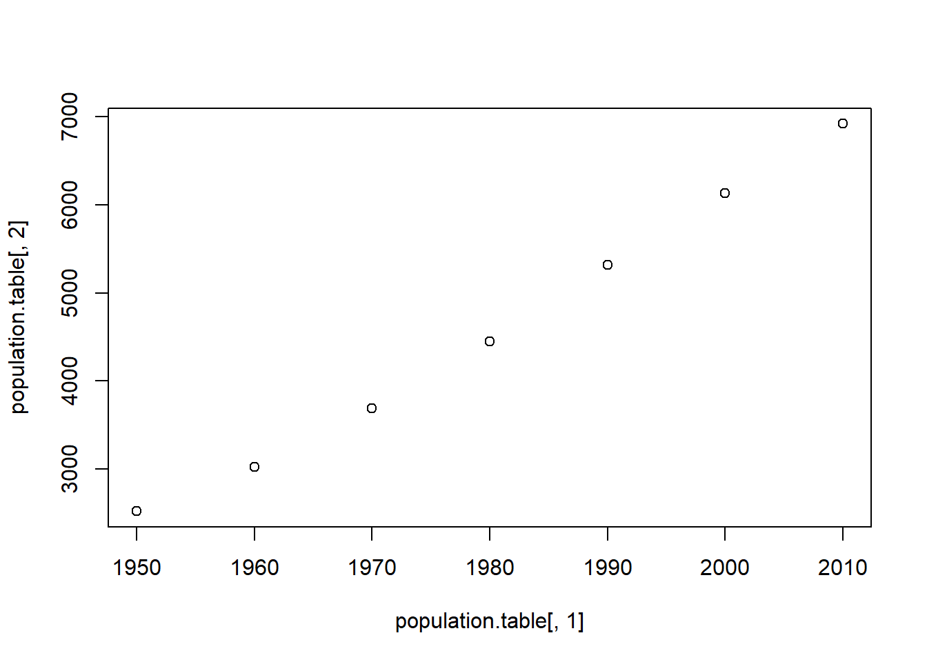
Because we are telling x,y coordinates for every point, the vectors we feed in to the plot command have to be the same length.
#Uncomment the next line to see what happens when the two vectors are different lengths:
#plot(population.table[,1], population.table[-1,2])
That graph looks OK, but it’s not something we would want to present. We can use options in the plot command to improve some things.
First, we want an overall title and labels for the two axes:
plot(population.table[,1], population.table[,2],
     main="Global Population Growth",
     xlab="Year",
     ylab="Population (Millions)")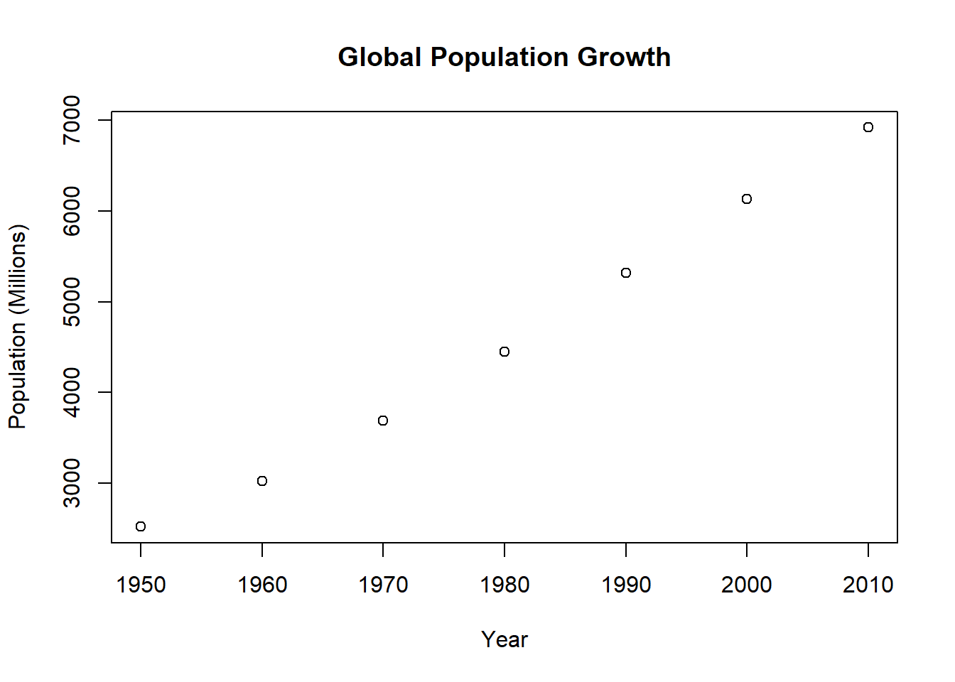
I’m not a big fan of these hollow dots, so we can also change the point “type”
plot(population.table[,1], population.table[,2],
     main="Global Population Growth",
     xlab="Year",
     ylab="Population (Millions)",
     pch=16)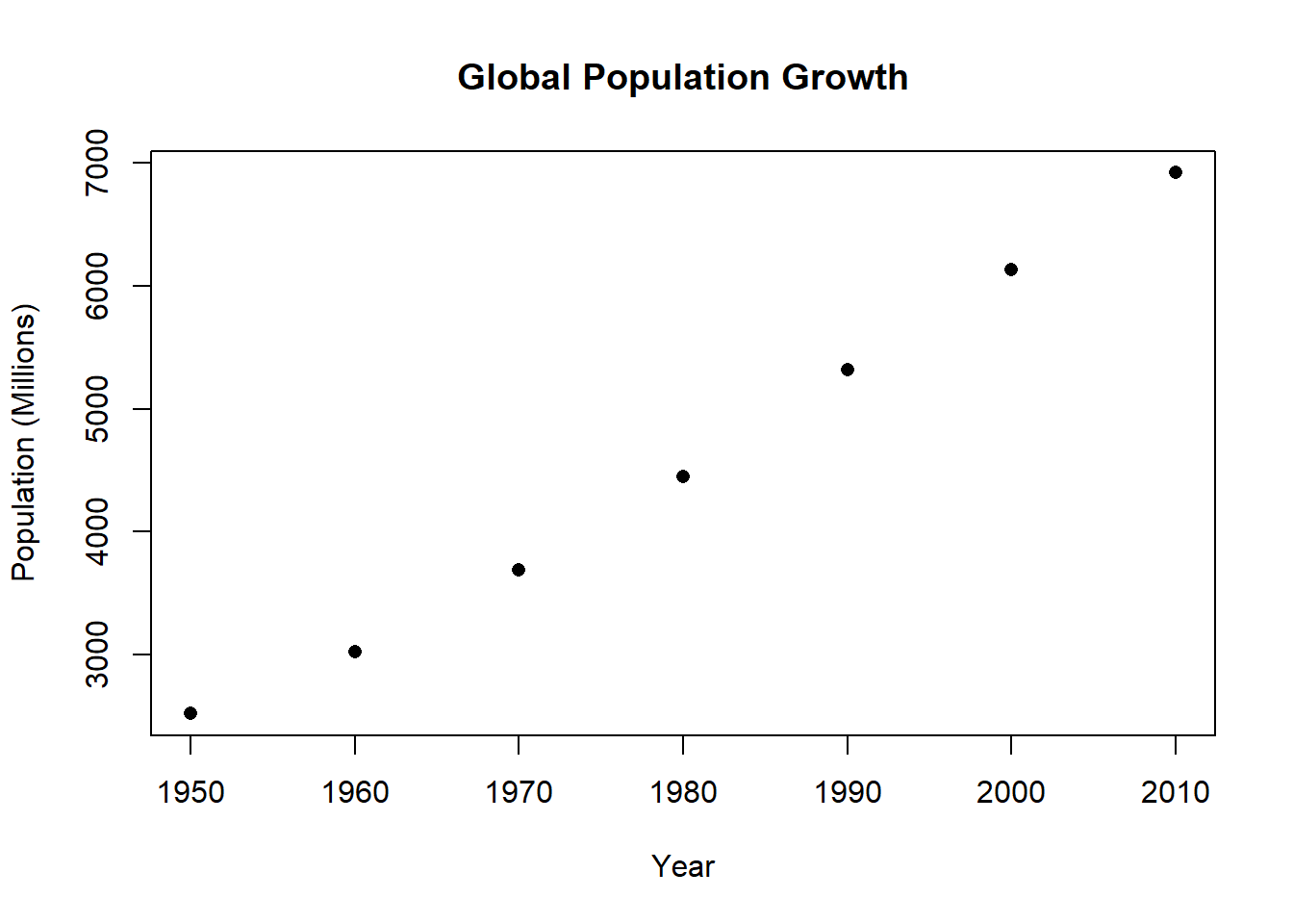
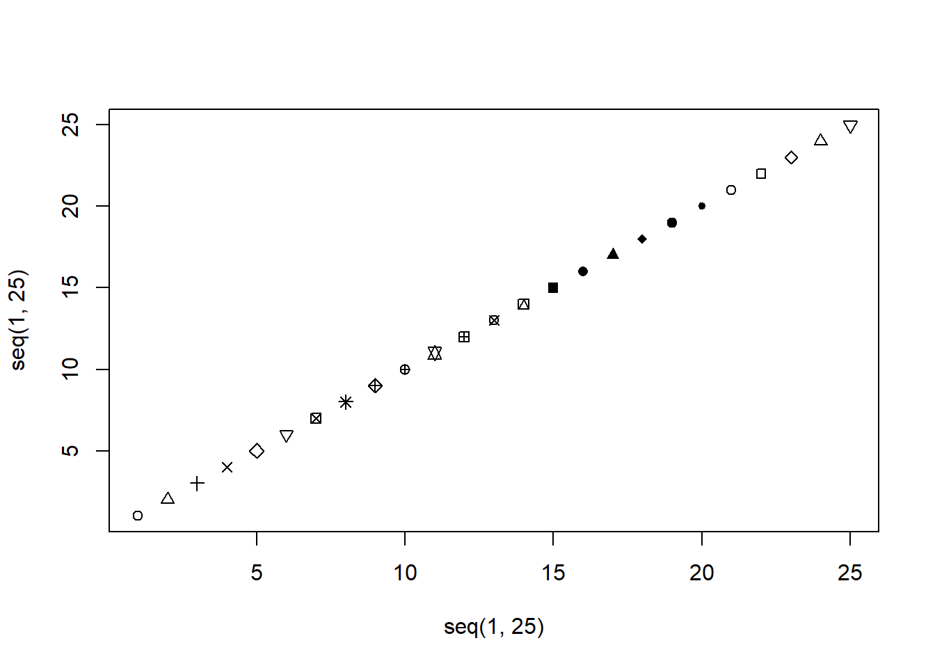
If you’re curious about all the point types….
What about some color?
#What about some color?

plot(population.table[,1], population.table[,2],
     main="Global Population Growth",
     xlab="Year",
     ylab="Population (Millions)",
     pch=16,
     col="darkorange")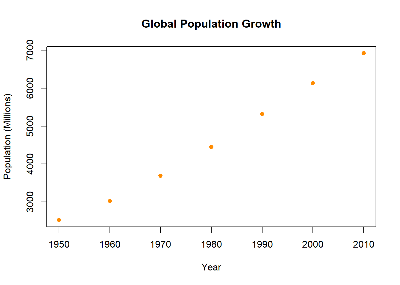
Here is a chart of all the colors: https://www.nceas.ucsb.edu/sites/default/files/2020-04/colorPaletteCheatsheet.pdf
These points form a series: the point for 1960 is after the point for 1950; the point for 1970 is after that etc. Because of that it is appropriate to connect these points, we can do that with the type option.
#The graph "type" will give you different options
#p = points
#l = line
#b = both
#n = none
#By default it's "p" so if you want points you don't
#have to do anything

#But if we want dots with lines connecting...

plot(population.table[,1], population.table[,2],
     main="Global Population Growth",
     xlab="Year",
     ylab="Population (Millions)",
     pch=16,
     col="darkorange",
     type="b")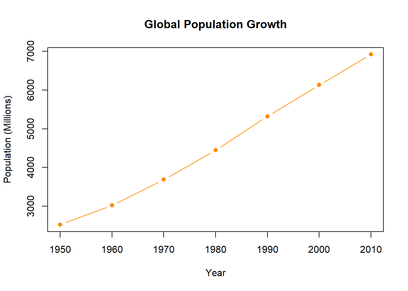
Let’s consider another graph with population rate on the x-axis and emissions on the y-axis:
plot(population.table[,3], population.table[,4],
xlab="Population Growth vs. 1950",
ylab="Co2 Emissions (billions of tons)",
main="Population Growth vs. Co2 Emissions",
pch=16)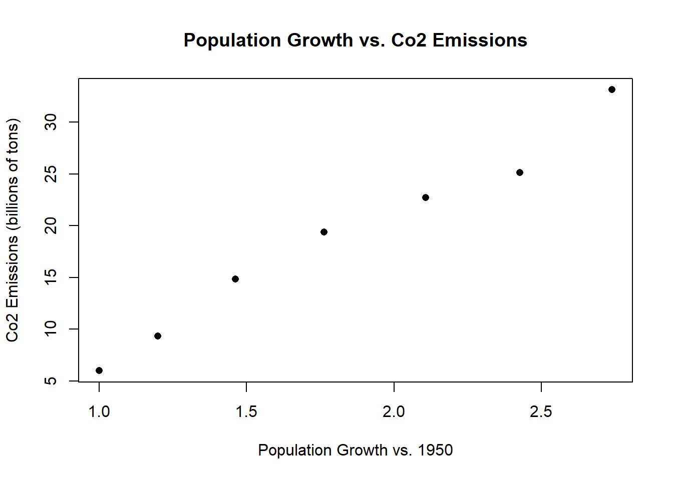 But it would be helpful for the viewers to know which point is which. What if instead of having these points we displayed the year information at the correct x,y coordinates?
There are large number of commands you can use to draw more information onto a figure after you have already set it up via the plot() command. One such command is text() which allows you to put text at specified coordinates.
With the text command we are saying, at the coordinates defined by the 3rd and 4th columns, write what is in the 1st column:
plot(population.table[,3], population.table[,4],
     xlab="Population Growth vs. 1950",
     ylab="Co2 Emissions (billions of tons)",
     main="Population Growth vs. Co2 Emissions",
     pch=16)
text(population.table[,3], population.table[,4],
     labels=population.table[,1])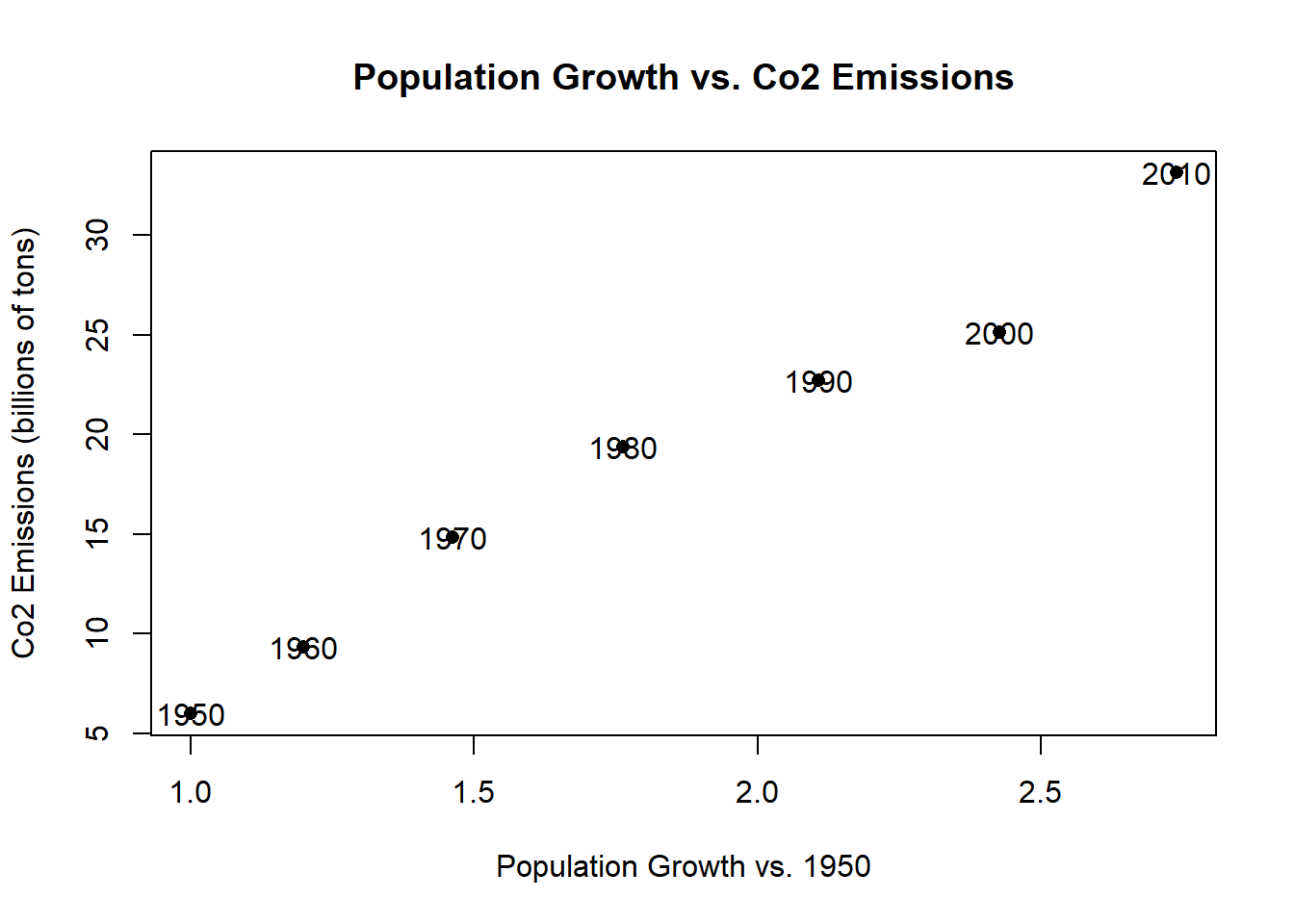
But now we are displaying both the points and the text. That’s not great! We could shift the text up by a little bit by adding to the y coordinates:
plot(population.table[,3], population.table[,4],
     xlab="Population Growth vs. 1950",
     ylab="Co2 Emissions (billions of tons)",
     main="Population Growth vs. Co2 Emissions", pch=16)
text(population.table[,3], population.table[,4]+2,
     labels=population.table[,1])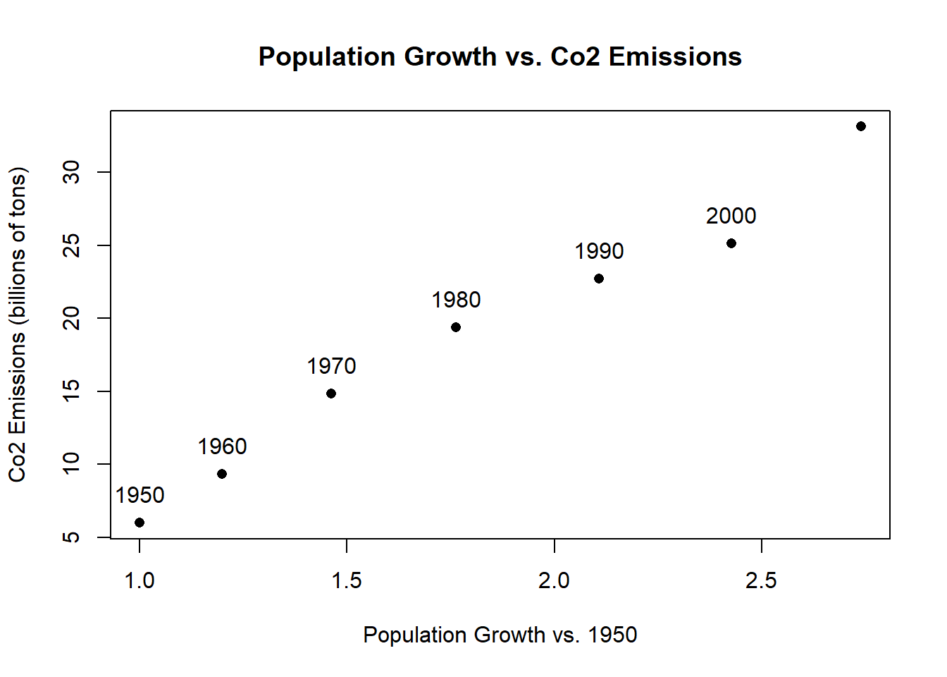
That looks good but our graph isn’t tall enough to get in one of the labels! We can adjust the axis size using the ylim= option:
plot(population.table[,3], population.table[,4],
     xlab="Population Growth vs. 1950",
     ylab="Co2 Emissions (billions of tons)",
     main="Population Growth vs. Co2 Emissions",
     pch=16,
     ylim=c(5,35))
text(population.table[,3], population.table[,4]+2,
     labels=population.table[,1])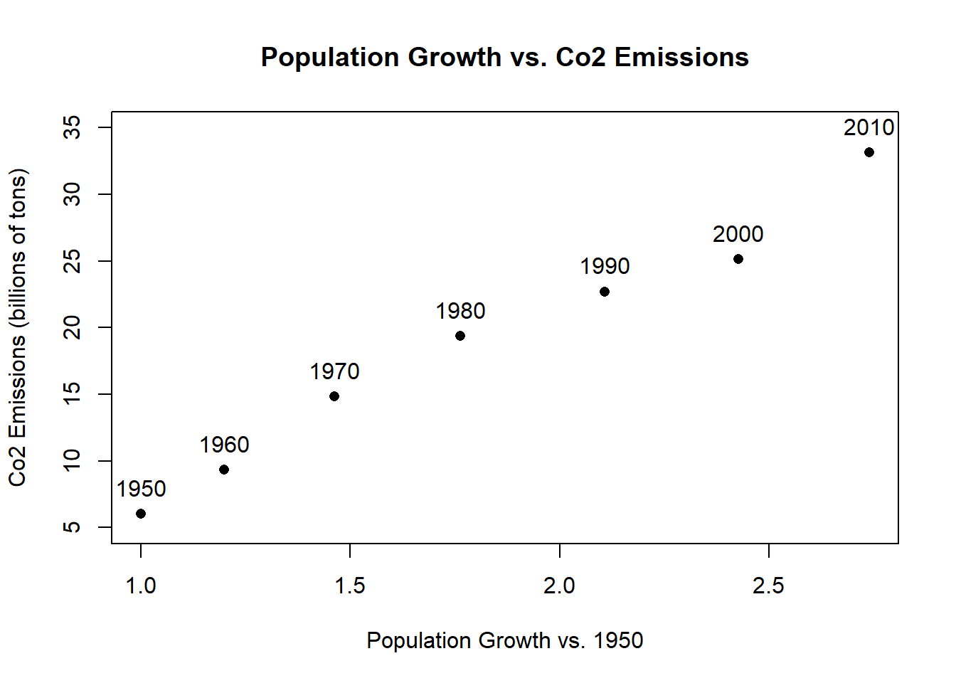
Another option is to adjust the type. You may have noticed that one of the types above is “none”. That will just plot no points, so we set up the graph without drawing the points, and then use the text command to fill them in!
plot(population.table[,3], population.table[,4],
     xlab="Population Growth vs. 1950",
     ylab="Co2 Emissions (billions of tons)",
     main="Population Growth vs. Co2 Emissions",
     pch=16,
     type = "n")
text(population.table[,3], population.table[,4],
     labels=population.table[,1])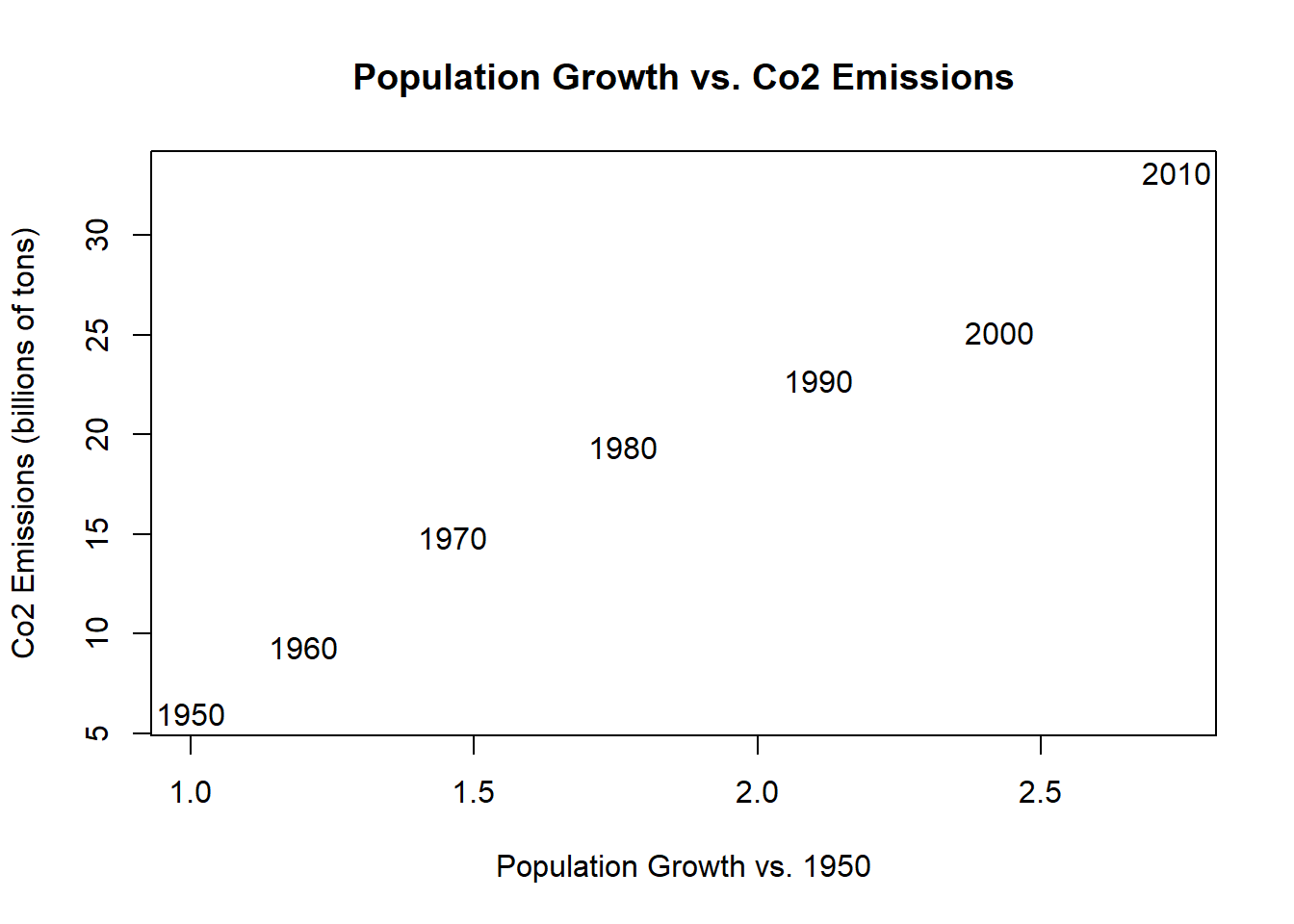
2.7 Condtional Logic
The first big extension to unlocking the power of R is thinking using “Conditional Logic. To get there, we first have to consider a special sort of variable class in R, the”boolean” variable. Boolean is just a fancy way of saying True or False.
If we give R some expressions that can be True or False, it will evaluate them:
2 == 1+1
#> [1] TRUE

1/2 == .5
#> [1] TRUE

2 == 3
#> [1] FALSE

2/3 == .6666
#> [1] FALSE
We can also use the double equals sign (or any other boolean operator) on vectors”
vec <- c(1,2,3,4,5)

vec == 3
#> [1] FALSE FALSE  TRUE FALSE FALSE
Other common boolean operators are greater than and less than:
2 > 3
#> [1] FALSE

2 < 3
#> [1] TRUE

vec > 3
#> [1] FALSE FALSE FALSE  TRUE  TRUE

vec >= 3
#> [1] FALSE FALSE  TRUE  TRUE  TRUE

vec <= 3
#> [1]  TRUE  TRUE  TRUE FALSE FALSE
Something that ends up being very helpful down the road for us is that R treats Trues as being equal to 1 and Falses be equal to 0. That means that we can quickly figure out how many items in a vector are true:
sum(vec >= 3)
#> [1] 3
Moreso, it lets us take advantage of the fast that the mean of a vector of 1’s and 0’s is equal to the probability that the vector is equal to 1.
mean(vec >= 3)
#> [1] 0.6
Another key boolean operator is the exclamation point, which negates logical statements.
2 == 3 #FALSE
#> [1] FALSE

2 != 3 #TRUE
#> [1] TRUE

!(2 == 3) #TRUE. essentially the same as the one above
#> [1] TRUE

2 > 3 #FALSE
#> [1] FALSE

!(2 > 3) #TRUE
#> [1] TRUE

!c(T, F, T,T,T, F)
#> [1] FALSE  TRUE FALSE FALSE FALSE  TRUE
So what’s the point of all of this?
The key thing is that we can put T/F statements inside square brackets to help us to subset data. Specifically, R will only return items in positions for which the boolean variable is true.
Return the values where emissions are less than 20:
emissions <- population.table[,4]
emissions
#> [1]  6.00  9.33 14.83 19.37 22.70 25.12 33.13
emissions<20
#> [1]  TRUE  TRUE  TRUE  TRUE FALSE FALSE FALSE
emissions[emissions<20]
#> [1]  6.00  9.33 14.83 19.37
Return the values where population is greater than 4000:
world.pop <- population.table[,2]

world.pop[world.pop>4000]
#> [1] 4449 5320 6127 6916
Perhaps more importantly, we can subset our entire data table based on a condition:
Return the data based on the conditions we specified:
#Emissions less than 20
population.table[population.table[,4]<20,]
#>      year world.pop pop.rate emissions
#> [1,] 1950      2525 1.000000      6.00
#> [2,] 1960      3026 1.198416      9.33
#> [3,] 1970      3691 1.461782     14.83
#> [4,] 1980      4449 1.761980     19.37

#World population less than 4000
population.table[population.table[,2]>4000,]
#>      year world.pop pop.rate emissions
#> [1,] 1980      4449 1.761980     19.37
#> [2,] 1990      5320 2.106931     22.70
#> [3,] 2000      6127 2.426535     25.12
#> [4,] 2010      6916 2.739010     33.13
This seems a bit silly right now where I can just visually see the rows that meet this criteria. Hold on for about 10 minutes and you will see why this is so helpful in large datasets.
We, of course, don’t have to rely on hand entered numbers for conditions, What if, instead, we want the rows where each of these variables are above their median values?
population.table[population.table[,4]> median(population.table[,4]),]
#>      year world.pop pop.rate emissions
#> [1,] 1990      5320 2.106931     22.70
#> [2,] 2000      6127 2.426535     25.12
#> [3,] 2010      6916 2.739010     33.13

population.table[population.table[,2]> median(population.table[,2]),]
#>      year world.pop pop.rate emissions
#> [1,] 1990      5320 2.106931     22.70
#> [2,] 2000      6127 2.426535     25.12
#> [3,] 2010      6916 2.739010     33.13
In this way it’s pretty straightforward to subset a matrix based on a condition.
An important extension to this is the ability to have more than one condition. For this we have both an AND and OR function.
For the AND function we use the ampersand:
(2 == 2) & (3 == 3) #TRUE
#> [1] TRUE

(2 == 2) & (3 == 2) #FALSE
#> [1] FALSE
The ‘OR’ operator is denoted by the pipe:
(2 == 2) | (3 == 2) #TRUE
#> [1] TRUE

(2 == 8) | (3 == 2) #FALSE
#> [1] FALSE
A helpful shortcut for seperating AND and OR functions is:
- With an AND function the whole statement is true if and only if all component statements are true.
- With an OR function the whole statement is true if any of the component statements are true.
Now return the rows of population table where world pop is greater than 4000 and emissions are greater than 20:
population.table[population.table[,2] > 4000 & population.table[,4] >20,]
#>      year world.pop pop.rate emissions
#> [1,] 1990      5320 2.106931     22.70
#> [2,] 2000      6127 2.426535     25.12
#> [3,] 2010      6916 2.739010     33.13
Does using OR give us a different result?
population.table[population.table[,2] > 4000 | population.table[,4] >20,]
#>      year world.pop pop.rate emissions
#> [1,] 1980      4449 1.761980     19.37
#> [2,] 1990      5320 2.106931     22.70
#> [3,] 2000      6127 2.426535     25.12
#> [4,] 2010      6916 2.739010     33.13
There is one other helpful boolean operator, which is the %in% operator.
This operator tells you if items in one number or character vector are contained in a second number of character vector.
So consider the confusing and overlapping band memberships of Buffalo Springfield, Crosby Stills and Nash, and Crosby Stills Nash and Young.
buffalo.springfield <- c("stills", "martin","palmer","furay","young")
csn <- c("crosby","stills","nash")
csny <- c("crosby","stills","nash","young")
The %in% operator will tell me: which members of Buffalo Springfield were in CSN?
buffalo.springfield %in% csn
#> [1]  TRUE FALSE FALSE FALSE FALSE
buffalo.springfield %in% csny
#> [1]  TRUE FALSE FALSE FALSE  TRUE

buffalo.springfield[buffalo.springfield %in% csny]
#> [1] "stills" "young"

#What members of Buffalo Springfield weren't in CSNY?
buffalo.springfield[!(buffalo.springfield %in% csny)]
#> [1] "martin" "palmer" "furay"
2.8 Data Frames
Let’s say I wanted to add a variable which is my subjective rating of the music quality of each of these decades, which can be “good” “bad” or “meh”:
music <- c("meh","good","meh","bad","good","bad","good")Let’s try to add this to our little dataset
population.table2 <- cbind(population.table, music)What did we get?
population.table2
#>      year   world.pop pop.rate           emissions music
#> [1,] "1950" "2525"    "1"                "6"       "meh"
#> [2,] "1960" "3026"    "1.19841584158416" "9.33"    "good"
#> [3,] "1970" "3691"    "1.46178217821782" "14.83"   "meh"
#> [4,] "1980" "4449"    "1.76198"          "19.37"   "bad"
#> [5,] "1990" "5320"    "2.10693069306931" "22.7"    "good"
#> [6,] "2000" "6127"    "2.42653465346535" "25.12"   "bad"
#> [7,] "2010" "6916"    "2.7390099009901"  "33.13"   "good"
On first inspection this looks fine, but note that everything here is in quotation marks. We know that quotation marks signify that R is treating information as “character”. If we try to take the mean of the first column:
#mean(population.table2[,1])We will get an error because we are asking R to take the mean of something it considers words.
Trying to add a character vector into our simple matrix of data has revealed a key shortcoming: these simple matrices can only contain one type of data. The way we fix this is instead using a “data.frame” which is a special sort of matrix that allows us to be much more flexible in what we store. This is predominate way we store data in R.
We can use a very similar type of cbind command to bind these things as a data frame instead of as a simple matrix:
population.table <- cbind.data.frame(population.table,music)
population.table
#>   year world.pop pop.rate emissions music
#> 1 1950      2525 1.000000      6.00   meh
#> 2 1960      3026 1.198416      9.33  good
#> 3 1970      3691 1.461782     14.83   meh
#> 4 1980      4449 1.761980     19.37   bad
#> 5 1990      5320 2.106931     22.70  good
#> 6 2000      6127 2.426535     25.12   bad
#> 7 2010      6916 2.739010     33.13  good
We can now perform math on things that are numbers:
mean(population.table[,2])
#> [1] 4579.143
And we can perform character functions on things that are characters:
nchar(population.table[,5])
#> [1] 3 4 3 3 4 3 4
So now, can we determine the rows in which music was good or meh?
population.table[population.table[,5]=="good" | population.table[,5]=="meh",]
#>   year world.pop pop.rate emissions music
#> 1 1950      2525 1.000000      6.00   meh
#> 2 1960      3026 1.198416      9.33  good
#> 3 1970      3691 1.461782     14.83   meh
#> 5 1990      5320 2.106931     22.70  good
#> 7 2010      6916 2.739010     33.13  good
What if we wanted all the years that were bad?
For demonstration, note that we can do this:
population.table[!(population.table[,5]=="good" | population.table[,5]=="meh"),]
#>   year world.pop pop.rate emissions music
#> 4 1980      4449 1.761980     19.37   bad
#> 6 2000      6127 2.426535     25.12   bad
But really we would do:
population.table[population.table[,5]=="bad",]
#>   year world.pop pop.rate emissions music
#> 4 1980      4449 1.761980     19.37   bad
#> 6 2000      6127 2.426535     25.12   bad
What would happen if we did the original command with & instead of | ?
population.table[population.table[,5]=="good" & population.table[,5]=="meh",]
#> [1] year      world.pop pop.rate  emissions music
#> <0 rows> (or 0-length row.names)
Nothing, thinking through that command logically it doesn’t make much sense…
We can see in the environment that data frames get a special blue arrow that we can click to see the different variable names. Indeed, this is the other main benefit of the use of data frames. So far we
When we work with data are we really going to have to remember which column everything is all the time?? No, definitely not.
While it’s good to understand that R thinks about things having position as rows and columns, but in reality we are going to take advantage of the fact that dataframes allow us to name counties.
Let’s work with a slightly (much) bigger dataframe so that we can fully take advantage of their properties.
R has the ability to load data stored on your computer, which will be a key thing to learn down the road. However, for simplicity I have stored all the data for this class online. R can also load data directly from a link.
If we run the following command it will load in data for every county from the American Community Survey (ACS)
acs <- read.csv("https://raw.githubusercontent.com/marctrussler/IIS-Data/main/ACSCountyData.csv")Note that we have not just run read.csv() on its own, but have assigned the output to an object acs. If we had just run the command on it’s own R would have simply printed the information from that csv into the terminal. Not that helpful!
The file we’ve loaded is data on county demographics in the United States. Now we see that there is a special object in the environment “acs”
class(acs)
#> [1] "data.frame"
That blue arrow means that we can click on it and see what acs consists of. In this case this is the list all of the variable names
We can also click on the dataset and it will open in a new window for us to look at.
One important consideration in describing a dataset is the *unit of analysis**. This is a fancy way of asking: what are in the rows?In this case, the unit of analysis is a county.
Think about studying what makes good schools, for example. We could conceive of data that would have different units of analysis
Could study schools: funding, student per teacher, household income…
Could study individual classrooms within schools
Could study students within classrooms within schools
Understanding what the unit of analysis of your data is fundamental.
Here are some basic tools for understanding a data frame:
#What are the variable names?
names(acs)
#>  [1] "X"                       "county.fips"
#>  [3] "county.name"             "state.full"
#>  [5] "state.abbr"              "state.alpha"
#>  [7] "state.icpsr"             "census.region"
#>  [9] "population"              "population.density"
#> [11] "percent.senior"          "percent.white"
#> [13] "percent.black"           "percent.asian"
#> [15] "percent.amerindian"      "percent.less.hs"
#> [17] "percent.college"         "unemployment.rate"
#> [19] "median.income"           "gini"
#> [21] "median.rent"             "percent.child.poverty"
#> [23] "percent.adult.poverty"   "percent.car.commute"
#> [25] "percent.transit.commute" "percent.bicycle.commute"
#> [27] "percent.walk.commute"    "average.commute.time"
#> [29] "percent.no.insurance"

#What do the first six rows of data look like?
head(acs)
#>   X county.fips     county.name state.full state.abbr
#> 1 1        1055   Etowah County    Alabama         AL
#> 2 2        1133  Winston County    Alabama         AL
#> 3 3        1053 Escambia County    Alabama         AL
#> 4 4        1001  Autauga County    Alabama         AL
#> 5 5        1003  Baldwin County    Alabama         AL
#> 6 6        1005  Barbour County    Alabama         AL
#>   state.alpha state.icpsr census.region population
#> 1           1          41         south     102939
#> 2           1          41         south      23875
#> 3           1          41         south      37328
#> 4           1          41         south      55200
#> 5           1          41         south     208107
#> 6           1          41         south      25782
#>   population.density percent.senior percent.white
#> 1          192.30800       18.33804      80.34856
#> 2           38.94912       21.05550      96.33927
#> 3           39.49123       17.34891      61.87045
#> 4           92.85992       14.58333      76.87862
#> 5          130.90190       19.54043      86.26620
#> 6           29.13214       17.97378      47.38189
#>   percent.black percent.asian percent.amerindian
#> 1    15.7491330     0.7179009          0.7295583
#> 2     0.3769634     0.1298429          0.3895288
#> 3    31.9331333     0.3616588          3.8496571
#> 4    19.1394928     1.0289855          0.2880435
#> 5     9.4970376     0.8072770          0.7313545
#> 6    47.5758281     0.3723528          0.2792646
#>   percent.less.hs percent.college unemployment.rate
#> 1       15.483020        17.73318          6.499382
#> 2       21.851723        13.53585          7.597536
#> 3       18.455613        12.65935         13.461675
#> 4       11.311414        27.68929          4.228036
#> 5        9.735422        31.34588          4.444240
#> 6       26.968580        12.21592          9.524798
#>   median.income   gini median.rent percent.child.poverty
#> 1         44023 0.4483         669              30.00183
#> 2         38504 0.4517         525              23.91744
#> 3         35000 0.4823         587              33.89582
#> 4         58786 0.4602         966              22.71976
#> 5         55962 0.4609         958              13.38019
#> 6         34186 0.4731         590              47.59704
#>   percent.adult.poverty percent.car.commute
#> 1              15.42045            94.28592
#> 2              15.83042            94.63996
#> 3              23.50816            98.54988
#> 4              14.03953            95.15310
#> 5              10.37312            91.71079
#> 6              25.40757            94.22581
#>   percent.transit.commute percent.bicycle.commute
#> 1              0.20813669              0.08470679
#> 2              0.38203288              0.00000000
#> 3              0.00000000              0.06667222
#> 4              0.10643524              0.05731128
#> 5              0.08969591              0.05797419
#> 6              0.25767159              0.00000000
#>   percent.walk.commute average.commute.time
#> 1            0.8373872                   24
#> 2            0.3473026                   29
#> 3            0.4250354                   23
#> 4            0.6263304                   26
#> 5            0.6956902                   27
#> 6            2.1316468                   23
#>   percent.no.insurance
#> 1            10.357590
#> 2            12.150785
#> 3            14.308294
#> 4             7.019928
#> 5            10.025612
#> 6             9.921651

#What do the last six rows of data look like?
tail(acs)
#>         X county.fips       county.name state.full
#> 3137 3137       56031     Platte County    Wyoming
#> 3138 3138       56033   Sheridan County    Wyoming
#> 3139 3139       56035   Sublette County    Wyoming
#> 3140 3140       56037 Sweetwater County    Wyoming
#> 3141 3141       56039      Teton County    Wyoming
#> 3142 3142       56041      Uinta County    Wyoming
#>      state.abbr state.alpha state.icpsr census.region
#> 3137         WY          50          68          west
#> 3138         WY          50          68          west
#> 3139         WY          50          68          west
#> 3140         WY          50          68          west
#> 3141         WY          50          68          west
#> 3142         WY          50          68          west
#>      population population.density percent.senior
#> 3137       8673           4.166810       23.44056
#> 3138      30012          11.893660       19.63881
#> 3139       9951           2.036434       16.72194
#> 3140      44117           4.231043       10.70109
#> 3141      23059           5.769299       13.59556
#> 3142      20609           9.899982       12.12092
#>      percent.white percent.black percent.asian
#> 3137      94.81148    0.01153004     0.6802721
#> 3138      95.07530    0.50979608     0.7030521
#> 3139      96.25163    0.00000000     0.1205909
#> 3140      93.12510    0.80241177     0.6324093
#> 3141      90.34217    1.18825621     1.2229498
#> 3142      93.41550    0.09704498     0.1067495
#>      percent.amerindian percent.less.hs percent.college
#> 3137         0.08071025        6.589393        21.73706
#> 3138         1.22617620        4.801207        29.98632
#> 3139         0.43211738        3.676471        25.24510
#> 3140         1.68189133        8.996576        22.03438
#> 3141         0.33392602        5.581450        57.37008
#> 3142         0.77635984        7.231901        15.44715
#>      unemployment.rate median.income   gini median.rent
#> 3137          2.666667         47096 0.4635         746
#> 3138          2.685430         58521 0.4383         809
#> 3139          3.409091         78680 0.3580         980
#> 3140          5.196641         73008 0.4127         868
#> 3141          1.445584         83831 0.4879        1339
#> 3142          6.054630         58235 0.4002         664
#>      percent.child.poverty percent.adult.poverty
#> 3137             20.304569             10.058188
#> 3138              6.346244              6.317891
#> 3139             10.041667              8.343327
#> 3140             14.092187             11.206294
#> 3141              4.212911              8.344662
#> 3142             15.980066             11.091579
#>      percent.car.commute percent.transit.commute
#> 3137            85.61220               0.6193425
#> 3138            87.57592               0.1214739
#> 3139            86.50675               0.3373313
#> 3140            89.88532               2.7568807
#> 3141            72.18383               4.0541503
#> 3142            92.80077               3.6049488
#>      percent.bicycle.commute percent.walk.commute
#> 3137               0.8575512            4.1686517
#> 3138               0.4251586            2.7534080
#> 3139               0.5997001            4.9100450
#> 3140               0.2522936            3.5045872
#> 3141               3.0495191           12.8678304
#> 3142               0.3306314            0.8532423
#>      average.commute.time percent.no.insurance
#> 3137                   17             9.927361
#> 3138                   16             9.542850
#> 3139                   20            13.365491
#> 3140                   20            11.877508
#> 3141                   15             9.996097
#> 3142                   21            12.125770

#Basic summary stats for all variables:
summary(acs)
#>        X           county.fips    county.name
#>  Min.   :   1.0   Min.   : 1001   Length:3142
#>  1st Qu.: 786.2   1st Qu.:18178   Class :character
#>  Median :1571.5   Median :29176   Mode  :character
#>  Mean   :1571.5   Mean   :30384
#>  3rd Qu.:2356.8   3rd Qu.:45081
#>  Max.   :3142.0   Max.   :56045
#>
#>   state.full         state.abbr         state.alpha
#>  Length:3142        Length:3142        Min.   : 1.00
#>  Class :character   Class :character   1st Qu.:14.00
#>  Mode  :character   Mode  :character   Median :25.00
#>                                        Mean   :26.34
#>                                        3rd Qu.:40.00
#>                                        Max.   :50.00
#>                                        NA's   :1
#>   state.icpsr    census.region        population
#>  Min.   : 1.00   Length:3142        Min.   :      75
#>  1st Qu.:32.00   Class :character   1st Qu.:   10948
#>  Median :43.00   Mode  :character   Median :   25736
#>  Mean   :41.45                      Mean   :  102770
#>  3rd Qu.:51.00                      3rd Qu.:   67209
#>  Max.   :82.00                      Max.   :10098052
#>
#>  population.density percent.senior   percent.white
#>  Min.   :    0.04   Min.   : 3.799   Min.   :  3.891
#>  1st Qu.:   16.69   1st Qu.:15.448   1st Qu.: 76.631
#>  Median :   44.72   Median :18.038   Median : 89.636
#>  Mean   :  270.68   Mean   :18.364   Mean   : 83.055
#>  3rd Qu.:  116.71   3rd Qu.:20.805   3rd Qu.: 95.065
#>  Max.   :72052.96   Max.   :55.596   Max.   :100.000
#>
#>  percent.black     percent.asian    percent.amerindian
#>  Min.   : 0.0000   Min.   : 0.000   Min.   : 0.0000
#>  1st Qu.: 0.6738   1st Qu.: 0.291   1st Qu.: 0.1712
#>  Median : 2.2673   Median : 0.606   Median : 0.3498
#>  Mean   : 9.0596   Mean   : 1.373   Mean   : 1.9671
#>  3rd Qu.:10.1602   3rd Qu.: 1.315   3rd Qu.: 0.8419
#>  Max.   :87.4123   Max.   :42.511   Max.   :92.4799
#>
#>  percent.less.hs  percent.college unemployment.rate
#>  Min.   : 1.183   Min.   : 0.00   Min.   : 0.000
#>  1st Qu.: 8.755   1st Qu.:15.00   1st Qu.: 3.982
#>  Median :12.081   Median :19.25   Median : 5.447
#>  Mean   :13.409   Mean   :21.57   Mean   : 5.774
#>  3rd Qu.:17.184   3rd Qu.:25.57   3rd Qu.: 7.073
#>  Max.   :66.344   Max.   :78.53   Max.   :28.907
#>                                   NA's   :1
#>  median.income         gini         median.rent
#>  Min.   : 20188   Min.   :0.2567   Min.   : 318
#>  1st Qu.: 42480   1st Qu.:0.4210   1st Qu.: 622
#>  Median : 49888   Median :0.4432   Median : 700
#>  Mean   : 51583   Mean   :0.4454   Mean   : 757
#>  3rd Qu.: 57611   3rd Qu.:0.4673   3rd Qu.: 829
#>  Max.   :136268   Max.   :0.6647   Max.   :2158
#>  NA's   :1        NA's   :1        NA's   :3
#>  percent.child.poverty percent.adult.poverty
#>  Min.   : 0.00         Min.   : 0.00
#>  1st Qu.:14.26         1st Qu.:10.42
#>  Median :20.32         Median :14.18
#>  Mean   :21.49         Mean   :15.05
#>  3rd Qu.:26.90         3rd Qu.:18.44
#>  Max.   :72.59         Max.   :52.49
#>  NA's   :2             NA's   :1
#>  percent.car.commute percent.transit.commute
#>  Min.   : 7.947      Min.   : 0.0000
#>  1st Qu.:87.726      1st Qu.: 0.1081
#>  Median :91.161      Median : 0.3639
#>  Mean   :89.367      Mean   : 0.9812
#>  3rd Qu.:93.448      3rd Qu.: 0.8106
#>  Max.   :99.084      Max.   :61.9243
#>  NA's   :1           NA's   :1
#>  percent.bicycle.commute percent.walk.commute
#>  Min.   : 0.0000         Min.   : 0.000
#>  1st Qu.: 0.0000         1st Qu.: 1.333
#>  Median : 0.1405         Median : 2.240
#>  Mean   : 0.3308         Mean   : 3.175
#>  3rd Qu.: 0.3842         3rd Qu.: 3.734
#>  Max.   :10.9091         Max.   :53.784
#>  NA's   :1               NA's   :1
#>  average.commute.time percent.no.insurance
#>  Min.   : 5.00        Min.   : 1.524
#>  1st Qu.:20.00        1st Qu.: 6.060
#>  Median :23.00        Median : 8.933
#>  Mean   :23.57        Mean   : 9.811
#>  3rd Qu.:27.00        3rd Qu.:12.334
#>  Max.   :45.00        Max.   :45.518
#>  NA's   :2
We also might want to know the number of variables and observations.
nrow(acs)
#> [1] 3142

ncol(acs)
#> [1] 29

#Another way to use this is to use the dim() function which does both at the same time

dim(acs)
#> [1] 3142   29
The important part of data.frame is that we can now use the variable name to look at columns, instead of the column number
The key operator here is the $ sign. We can call any variable by using the dollar sign and its varriable name:
head(acs$population)
#> [1] 102939  23875  37328  55200 208107  25782
Note also that population is the 8th column in the dataset, so doing the above is literally the same as:
head(acs[,8])
#> [1] "south" "south" "south" "south" "south" "south"
Because acs$population is an individual row, we can use the square brackets to index that variable:
acs$population[2:4]
#> [1] 23875 37328 55200
We can easily run the same sort of statistics on these variables:
mean(acs$population)
#> [1] 102769.9

max(acs$population)
#> [1] 10098052

median(acs$population)
#> [1] 25736
We are also able to perform arithmetic on these variables the same as we’ve been doing before. For example, if we want population in thousands:
head(acs$population/1000)
#> [1] 102.939  23.875  37.328  55.200 208.107  25.782
But we can do more than this, using the assignment operator we can create a new variable in our dataset that saves this information:
acs$pop.1000 <- acs$population/1000

head(acs$pop.1000)
#> [1] 102.939  23.875  37.328  55.200 208.107  25.782
This is just like how we created a vector above, but now we are creating it within a dataframe.
What if we want the area in square miles of a county? Right now we just have population and density. But because:
\[ density = pop/area\\ area =pop/density \]
acs$area <- acs$population/acs$population.density
head(acs$area)
#> [1]  535.2819  612.9792  945.2225  594.4438 1589.7936
#> [6]  885.0019
Or create a percent non white or black variable
acs$perc.non.white.black <- 100 - (acs$percent.white + acs$percent.black)
head(acs$perc.non.white.black)
#> [1] 3.902311 3.283770 6.196421 3.981884 4.236763 5.042278
For a given variable, we might be interested in learning what all of the possible values are
head(acs$census.region)
#> [1] "south" "south" "south" "south" "south" "south"

unique(acs$census.region)
#> [1] "south"     "west"      "northeast" "midwest"
That gives us all the unique values, but not how relatively common each of these categories are. We can answer this second question with table()
table(acs$census.region)
#>
#>   midwest northeast     south      west
#>      1055       217      1422       448
If you want these to be proportions (we are going to want proportions a lot in this class!), you can wrap that whole thing with prop.table()
prop.table(table(acs$census.region))
#>
#>    midwest  northeast      south       west
#> 0.33577339 0.06906429 0.45257798 0.14258434
Remember, though, these commands are only applicable to variables with a discrete number of possible values. It is pretty useless to do:
A final important command is the order function. For a given variable, this function will return the row numbers sorted from smallest to largest. This will print out all of the row numbers in order, so to just see the first 6 (the smallest 6 counties) we can use the head command.
So row 551 contains the observation with the lowest population
acs[551,]
#>       X county.fips    county.name state.full state.abbr
#> 551 551       15005 Kalawao County     Hawaii         HI
#>     state.alpha state.icpsr census.region population
#> 551          11          82          west         75
#>     population.density percent.senior percent.white
#> 551           6.254478             16      21.33333
#>     percent.black percent.asian percent.amerindian
#> 551      2.666667            28           2.666667
#>     percent.less.hs percent.college unemployment.rate
#> 551        13.04348        24.63768                 0
#>     median.income   gini median.rent percent.child.poverty
#> 551         61875 0.3589         863                    NA
#>     percent.adult.poverty percent.car.commute
#> 551              11.86441            43.63636
#>     percent.transit.commute percent.bicycle.commute
#> 551                       0                10.90909
#>     percent.walk.commute average.commute.time
#> 551                   40                    5
#>     percent.no.insurance pop.1000     area
#> 551             2.666667    0.075 11.99141
#>     perc.non.white.black
#> 551                   76
And we see it’s Kalawao County with 75 people
What about the largest county?
We could look at the tail:
tail(order(acs$population))
#> [1]  218  225  106 2546  655  207
acs[207,]
#>       X county.fips        county.name state.full
#> 207 207        6037 Los Angeles County California
#>     state.abbr state.alpha state.icpsr census.region
#> 207         CA           5          71          west
#>     population population.density percent.senior
#> 207   10098052           2488.312       12.86661
#>     percent.white percent.black percent.asian
#> 207      51.36495      8.159861      14.55695
#>     percent.amerindian percent.less.hs percent.college
#> 207          0.6984218         21.3384        31.80899
#>     unemployment.rate median.income   gini median.rent
#> 207          6.833541         64251 0.5022        1390
#>     percent.child.poverty percent.adult.poverty
#> 207              22.47003              14.28525
#>     percent.car.commute percent.transit.commute
#> 207             83.4639                6.210588
#>     percent.bicycle.commute percent.walk.commute
#> 207               0.8323332             2.716764
#>     average.commute.time percent.no.insurance pop.1000
#> 207                   31             10.76106 10098.05
#>         area perc.non.white.black
#> 207 4058.194             40.47519
So row 551 contains the observation with the lowest population
A more flexible way to answer this question is with the which() command. With this command you can feed it any logical statement and it will return the rows for which it is true.
For example, where are the places where median income is at its max and min?
which(acs$median.income==max(acs$median.income,na.rm=T))
#> [1] 2835
acs[2835,]
#>         X county.fips    county.name state.full state.abbr
#> 2835 2835       51107 Loudoun County   Virginia         VA
#>      state.alpha state.icpsr census.region population
#> 2835          46          40         south     385143
#>      population.density percent.senior percent.white
#> 2835           746.7396       8.637052      66.15387
#>      percent.black percent.asian percent.amerindian
#> 2835      7.460865      17.97306          0.2586052
#>      percent.less.hs percent.college unemployment.rate
#> 2835        6.486335        60.79087          3.489436
#>      median.income   gini median.rent percent.child.poverty
#> 2835        136268 0.3859        1813              3.771955
#>      percent.adult.poverty percent.car.commute
#> 2835              3.505573            85.70692
#>      percent.transit.commute percent.bicycle.commute
#> 2835                4.165227                0.191762
#>      percent.walk.commute average.commute.time
#> 2835             1.733159                   34
#>      percent.no.insurance pop.1000     area
#> 2835             6.161608  385.143 515.7661
#>      perc.non.white.black
#> 2835             26.38526

which(acs$median.income==min(acs$median.income,na.rm=T))
#> [1] 1435
acs[1435,]
#>         X county.fips      county.name  state.full
#> 1435 1435       28063 Jefferson County Mississippi
#>      state.abbr state.alpha state.icpsr census.region
#> 1435         MS          24          46         south
#>      population population.density percent.senior
#> 1435       7346           14.12874       14.90607
#>      percent.white percent.black percent.asian
#> 1435      13.32698      85.89709     0.4492241
#>      percent.amerindian percent.less.hs percent.college
#> 1435          0.1497414        25.18977          15.002
#>      unemployment.rate median.income   gini median.rent
#> 1435          7.535944         20188 0.4982         423
#>      percent.child.poverty percent.adult.poverty
#> 1435              65.40284               46.8599
#>      percent.car.commute percent.transit.commute
#> 1435            95.28509                       0
#>      percent.bicycle.commute percent.walk.commute
#> 1435                       0              1.91886
#>      average.commute.time percent.no.insurance pop.1000
#> 1435                   24             15.80452    7.346
#>          area perc.non.white.black
#> 1435 519.9331            0.7759325

which(acs$median.income==median(acs$median.income,na.rm=T))
#> [1] 1077
acs[1077,]
#>         X county.fips    county.name state.full state.abbr
#> 1077 1077       21079 Garrard County   Kentucky         KY
#>      state.alpha state.icpsr census.region population
#> 1077          17          51         south      17328
#>      population.density percent.senior percent.white
#> 1077           75.30685       17.44575      96.12188
#>      percent.black percent.asian percent.amerindian
#> 1077      1.108033     0.1385042          0.4039705
#>      percent.less.hs percent.college unemployment.rate
#> 1077        20.09433        16.79271          5.989682
#>      median.income   gini median.rent percent.child.poverty
#> 1077         49888 0.4325         689               25.1379
#>      percent.adult.poverty percent.car.commute
#> 1077              15.12774            92.42466
#>      percent.transit.commute percent.bicycle.commute
#> 1077               0.1780822                       0
#>      percent.walk.commute average.commute.time
#> 1077            0.3972603                   34
#>      percent.no.insurance pop.1000     area
#> 1077             7.450369   17.328 230.0986
#>      perc.non.white.black
#> 1077             2.770083
2.9 Conditional logic in dataframes
We’ve worked a lot to learn how to use square brackets in simple matrices. This logic directly extends to working with data frames.
For example, what are the first 10 rows in acs?
acs[1:10,]
#>     X county.fips     county.name state.full state.abbr
#> 1   1        1055   Etowah County    Alabama         AL
#> 2   2        1133  Winston County    Alabama         AL
#> 3   3        1053 Escambia County    Alabama         AL
#> 4   4        1001  Autauga County    Alabama         AL
#> 5   5        1003  Baldwin County    Alabama         AL
#> 6   6        1005  Barbour County    Alabama         AL
#> 7   7        1007     Bibb County    Alabama         AL
#> 8   8        1009   Blount County    Alabama         AL
#> 9   9        1011  Bullock County    Alabama         AL
#> 10 10        1013   Butler County    Alabama         AL
#>    state.alpha state.icpsr census.region population
#> 1            1          41         south     102939
#> 2            1          41         south      23875
#> 3            1          41         south      37328
#> 4            1          41         south      55200
#> 5            1          41         south     208107
#> 6            1          41         south      25782
#> 7            1          41         south      22527
#> 8            1          41         south      57645
#> 9            1          41         south      10352
#> 10           1          41         south      20025
#>    population.density percent.senior percent.white
#> 1           192.30800       18.33804      80.34856
#> 2            38.94912       21.05550      96.33927
#> 3            39.49123       17.34891      61.87045
#> 4            92.85992       14.58333      76.87862
#> 5           130.90190       19.54043      86.26620
#> 6            29.13214       17.97378      47.38189
#> 7            36.19020       16.25161      76.65468
#> 8            89.39555       17.75176      95.50525
#> 9            16.62156       15.61051      21.98609
#> 10           25.77756       19.00624      52.00499
#>    percent.black percent.asian percent.amerindian
#> 1     15.7491330     0.7179009        0.729558282
#> 2      0.3769634     0.1298429        0.389528796
#> 3     31.9331333     0.3616588        3.849657094
#> 4     19.1394928     1.0289855        0.288043478
#> 5      9.4970376     0.8072770        0.731354544
#> 6     47.5758281     0.3723528        0.279264603
#> 7     22.2754916     0.1642473        0.035512940
#> 8      1.4953595     0.3434817        0.244600572
#> 9     76.2461360     0.5409583        1.178516229
#> 10    45.2184769     1.1535581        0.009987516
#>    percent.less.hs percent.college unemployment.rate
#> 1        15.483020        17.73318          6.499382
#> 2        21.851723        13.53585          7.597536
#> 3        18.455613        12.65935         13.461675
#> 4        11.311414        27.68929          4.228036
#> 5         9.735422        31.34588          4.444240
#> 6        26.968580        12.21592          9.524798
#> 7        16.793409        11.48923          7.513989
#> 8        19.837485        12.64289          4.084475
#> 9        24.774775        13.30236         11.060948
#> 10       15.416187        16.09303          6.708471
#>    median.income   gini median.rent percent.child.poverty
#> 1          44023 0.4483         669              30.00183
#> 2          38504 0.4517         525              23.91744
#> 3          35000 0.4823         587              33.89582
#> 4          58786 0.4602         966              22.71976
#> 5          55962 0.4609         958              13.38019
#> 6          34186 0.4731         590              47.59704
#> 7          45340 0.4294         714              20.19043
#> 8          48695 0.4331         662              21.56789
#> 9          32152 0.5174         668              55.93465
#> 10         39109 0.4708         606              35.01215
#>    percent.adult.poverty percent.car.commute
#> 1               15.42045            94.28592
#> 2               15.83042            94.63996
#> 3               23.50816            98.54988
#> 4               14.03953            95.15310
#> 5               10.37312            91.71079
#> 6               25.40757            94.22581
#> 7               13.33063            95.50717
#> 8               12.85135            96.58597
#> 9               25.83914            91.42132
#> 10              22.37574            96.31870
#>    percent.transit.commute percent.bicycle.commute
#> 1               0.20813669              0.08470679
#> 2               0.38203288              0.00000000
#> 3               0.00000000              0.06667222
#> 4               0.10643524              0.05731128
#> 5               0.08969591              0.05797419
#> 6               0.25767159              0.00000000
#> 7               0.46564309              0.00000000
#> 8               0.14658597              0.00000000
#> 9               0.00000000              0.00000000
#> 10              0.00000000              0.00000000
#>    percent.walk.commute average.commute.time
#> 1             0.8373872                   24
#> 2             0.3473026                   29
#> 3             0.4250354                   23
#> 4             0.6263304                   26
#> 5             0.6956902                   27
#> 6             2.1316468                   23
#> 7             0.5537377                   29
#> 8             0.1891432                   35
#> 9             5.8375635                   29
#> 10            0.9267602                   24
#>    percent.no.insurance pop.1000      area
#> 1             10.357590  102.939  535.2819
#> 2             12.150785   23.875  612.9792
#> 3             14.308294   37.328  945.2225
#> 4              7.019928   55.200  594.4438
#> 5             10.025612  208.107 1589.7936
#> 6              9.921651   25.782  885.0019
#> 7              7.186931   22.527  622.4613
#> 8             10.934166   57.645  644.8308
#> 9             10.394127   10.352  622.8056
#> 10            10.012484   20.025  776.8385
#>    perc.non.white.black
#> 1              3.902311
#> 2              3.283770
#> 3              6.196421
#> 4              3.981884
#> 5              4.236763
#> 6              5.042278
#> 7              1.069827
#> 8              2.999393
#> 9              1.767774
#> 10             2.776529
acs.100 <- acs[1:10,]
Can we save a dataframe that is everything but the first 100 rows?
nrow(acs)
#> [1] 3142
#Harder:
acs.non.100 <- acs[101:3142,]

#Easier
acs.non.100 <- acs[-(1:100),]
More importantly, we can use the column names themselves and logical statements to reduce our datasets.
We have seen already that if we put some trues and falses in square brackets R will only return the items which are associated with trues.
To remind ourselves:
Extending that logic, can we produce a dataset that just has the counties in the south?
table(acs$census.region)
#>
#>   midwest northeast     south      west
#>      1055       217      1422       448
First write a logical statement that identifies those rows:
head(acs$census.region=="south",100)
#>   [1]  TRUE  TRUE  TRUE  TRUE  TRUE  TRUE  TRUE  TRUE  TRUE
#>  [10]  TRUE  TRUE  TRUE  TRUE  TRUE  TRUE  TRUE  TRUE  TRUE
#>  [19]  TRUE  TRUE  TRUE  TRUE  TRUE  TRUE  TRUE  TRUE  TRUE
#>  [28]  TRUE  TRUE  TRUE  TRUE  TRUE  TRUE  TRUE  TRUE  TRUE
#>  [37]  TRUE  TRUE  TRUE  TRUE  TRUE  TRUE  TRUE  TRUE  TRUE
#>  [46]  TRUE  TRUE  TRUE  TRUE  TRUE  TRUE  TRUE  TRUE  TRUE
#>  [55]  TRUE  TRUE  TRUE  TRUE  TRUE  TRUE  TRUE  TRUE  TRUE
#>  [64]  TRUE  TRUE  TRUE  TRUE FALSE FALSE FALSE FALSE FALSE
#>  [73] FALSE FALSE FALSE FALSE FALSE FALSE FALSE FALSE FALSE
#>  [82] FALSE FALSE FALSE FALSE FALSE FALSE FALSE FALSE FALSE
#>  [91] FALSE FALSE FALSE FALSE FALSE FALSE FALSE FALSE FALSE
#> [100] FALSE
Now put that logical statement in square brackets:
acs.south <- acs[acs$census.region=="south",]Note, again, the comma here with nothing after it. We are telling R: here are the rows we want to keep; also, we would like all of the columns.
What about counties where the population density is above the median population density?
median(acs$population.density)
#> [1] 44.71916

acs.highdensity <- acs[acs$population.density>median(acs$population.density),]
We can also use conditional logic when generating new variables.
Let’s say we wanted to create a new variable that splits counties into three types: - Urban (0-50 persons/mile) - Suburban (50-150 persons/mile) - Rural (>150 persons per mile)
We know that we can identify the rows in which these things are true:
head(acs$population.density<50)
#> [1] FALSE  TRUE  TRUE FALSE FALSE  TRUE
The way that we will think about creating a variable that indicates this is by first creating an empty variable:
acs$place.type <- NAAnd then re-coding the entries to that variable based on changing the values in a logical statement:
acs$place.type[acs$population.density<50]<- "rural"
acs$place.type[acs$population.density>=50 & acs$population.density<150] <-"suburban"
acs$place.type[acs$population.density>=150] <-"urban"

table(acs$place.type)
#>
#>    rural suburban    urban
#>     1689      793      660
What about if we want to create a dataset that just has the 4 electorally competitive mid-west states: MI,MN,OH,WI?
Again, we can accomplish this by writing a logical statement that would identify those rows :
acs.mw <- acs[acs$state.abbr=="MN" | acs$state.abbr=="WI" | acs$state.abbr=="MI" | acs$state.abbr=="OH",]But let’s not forget the %in% command! That can shortcut this significantly:
The things we can do with logical statements inside square brackets is pretty endless, but the same logic will always apply: thinking about making the rows we want to identify to come up as True.
2.10 Indicator Variables
There is a special type of variable that will be incredibly helpful for us in this course: indicator variables. As their name suggests, indicator variables indicate the presence of a particular feature.
Indicator variables take on the values of 0 or 1.
So if we were to create an indicator variable for a county being in the south:
acs$south <- NA
acs$south[acs$census.region=="south"]<- 1
acs$south[acs$census.region!="south" ]<- 0

table(acs$south)
#>
#>    0    1
#> 1720 1422
Or, slightly more complicated, an indicator variable for rural counties in the south:
acs$rural.south <- NA
acs$rural.south[acs$census.region=="south" & acs$place.type=="rural"]<- 1
acs$rural.south[acs$census.region!="south" | acs$place.type!="rural" ]<- 0

#What would have been wrong with:
#acs$census.region!="south" & acs$place.type!="rural"
#It would have set as false everywhere in the south
table(acs$rural.south)
#>
#>    0    1
#> 2480  662
Indicator variables are special (and important for this class) because of one particular mathematical quality: the mean of an indicator variable is equal to the proportion of the time that indicator variable is equal to 1.
We can see this really easily in a short example. Let’s say we have an indicator variable:
\[ \lbrace 0,1,1,0 \rbrace \]
I can visually see that 2 out of the 4 numbers are 1s. As such, the probability this vector takes on the value of 1 is .5, or 50%. And if we apply the formula for the mean:
\[ \frac{0+1+1+0}{4}= \frac{2}{4}=.5 \]
So what proportion of counties in America are rural counties in the south?
mean(acs$rural.south)
#> [1] 0.2106938
Approximately 21%.
What’s more, R has made this even easier for us. We learned about that R treats booleans as 1s and 0s. That means that we can shortcut what we did above significantly by just setting the variable equal to the logical statement!
2.11 For Loops
One of the most flexible tools in all coding languages is for() loops. In short: for() loops allow us to repeat the same code many, many, times.
This is particularly helpful for a class focused on probability. As we will see in the next chapter, what we mean by probability is the relative frequency of events if we repeat those events many, many times. With R, we can just actually simulate events many times using loops to give us insights into probability.
Above, we learned about how we can use the square brackets to give us conditional means.
For example we can easily get the mean population for all counties:
mean(acs$population)
#> [1] 102769.9
And if we want the mean population for just the counties in Alabama:
mean(acs$population[acs$state.abbr=="AL"])
#> [1] 72607.16
OK, but what if we wanted to do the same thing for all 50 states?
We could think about brute forcing it, subbing in the right two letter abbreviation and repeating the code 50 times:
mean(acs$population[acs$state.abbr=="AK"])
#> [1] 25466.07
mean(acs$population[acs$state.abbr=="AZ"])
#> [1] 463112.3
mean(acs$population[acs$state.abbr=="AR"])
#> [1] 39875.61
mean(acs$population[acs$state.abbr=="CA"])
#> [1] 674978.6
#
#
#
#
mean(acs$population[acs$state.abbr=="WI"])
#> [1] 80255.47
mean(acs$population[acs$state.abbr=="WY"])
#> [1] 25297.22
This is unwieldy! And I didn’t even do all of the states!
But notice something about the above block of code: most of the command on each line is exactly the same. All that we are changing in every line is what is in the quotations. WE are going from AL, to AL, to AZ…. all the way to WY.
So all we need is a method that allows us to run mean(acs$population[acs$state.abbr=="XX"]) 50 times, each time through changing XX to the next two-letter stabe abbreviation.
The way that we will accomplish this is with a for() loop.
Here is the basic setup for a for() loop:
for(i in 1:3){
  #CODE HERE
}
We can look at the for loop as having two parts. Everything from the start to the opening squiggly bracket are the instructions for the loop. It basically tells the loop how many times to repeat the same thing. “i” in this case is the variable that is going to change its value each time through the loop. Having this variable is what allows the loop to do something slightly different each time through the loop. The second part is whatever you put in between the squiggly brackets. This is the code that will be repeated again, and again the specified number of times.
Let’s put a simple bit of code in the loop to see how these work. I’m just going to put the command print(i) in the loop so that all the loop does is print the current value of i.
for(i in 1:3){
  print(i)
}
#> [1] 1
#> [1] 2
#> [1] 3
What a loop does is the following: on the first time through the loop it sets our variable (i) to the number 1. Literally. Anywhere we have the variable i, R will replace it with the integer 1. Once all the code has been executed and R reaches the closing squiggly bracket it goes back up the start. Now it will set i equal to 2. Anywhere in our code where there is currently the variable “i”, R will literally treat this as the integer 2. After it reaches the end of the code again, it will go back to the beginning and run the code again, this time making “i” equal to 3.
So the result of running this code is to simply print out the numbers 1, then 2, then 3.
To make this crystal clear, here is what code is literally being executed by R here. It is just the print command 3 times, the first time changing the variable i to the integer 1, the second time changing it to 2, and the third time changing it to 3.
Let’s take a second to think through the options at the start of this loop; everything that is contained in the opening parentheses.
Right now it says for(i in 1:3). This is saying: the variable that’s going to change everytime through the loop is called “i”, and the things we want to change it to is the sequence of numbers 1, 2, and then 3. Each of these things is customizable.
First, there is nothing special about “i”. We can name the variable that changes everytime through the script to anything we want.
So, for example, we can edit this same code to be for(batman in 1:3), and have the variable be called batman. And if we run this we get the exact same result.
for(batman in 1:3){
  print(batman)
}
#> [1] 1
#> [1] 2
#> [1] 3
This being said, it is convention to use the letter “i” as the indexing variable in a for loop. This is true across coding platforms so it’s a good idea to just use that.
Second, we can put any sort of vector into the second part. We can make it longer, for example, by running from 1 to 50.
for(i in 1:50){
  print(i)
}
#> [1] 1
#> [1] 2
#> [1] 3
#> [1] 4
#> [1] 5
#> [1] 6
#> [1] 7
#> [1] 8
#> [1] 9
#> [1] 10
#> [1] 11
#> [1] 12
#> [1] 13
#> [1] 14
#> [1] 15
#> [1] 16
#> [1] 17
#> [1] 18
#> [1] 19
#> [1] 20
#> [1] 21
#> [1] 22
#> [1] 23
#> [1] 24
#> [1] 25
#> [1] 26
#> [1] 27
#> [1] 28
#> [1] 29
#> [1] 30
#> [1] 31
#> [1] 32
#> [1] 33
#> [1] 34
#> [1] 35
#> [1] 36
#> [1] 37
#> [1] 38
#> [1] 39
#> [1] 40
#> [1] 41
#> [1] 42
#> [1] 43
#> [1] 44
#> [1] 45
#> [1] 46
#> [1] 47
#> [1] 48
#> [1] 49
#> [1] 50
We could also use the concatenate (or c() function) to give it a sequence of numbers to loop through. So here the first time through the loop i will be set equal to 2, the second time through it will be set equal to 15, and the third time through it will be set equal to 45.
Before you run this code, think: what code would the following produce?
Now let’s use our knowledge of for() loops to complete the task we set out: calculating the mean population for the counties in every state.
Let’s start by simply dropping in our code that we already have into our loop function.
for(i in 1:3){
  mean(acs$population[acs$state.abbr=="AL"])
}
Now, our target here is to change the state from AL, to AZ, to AR etc. each time through the loop. How can we use the functionality of loops, where R will sequentially change the variable i from 1, to 2, to 3 etc to accomplish that.
The way we are going to do that is to first create and save a vector of all the state abbreviations.
Using the unique() command, I can create a vector of all the state abbreviations. If we look at this, we now have a vector of all the possible state abbreviations. AL is first, AK is second, AZ is third.
states <- unique(acs$state.abbr)
states
#>  [1] "AL" "AK" "AZ" "AR" "CA" "CO" "CT" "DE" "DC" "FL" "GA"
#> [12] "HI" "ID" "IL" "IN" "IA" "KS" "KY" "LA" "ME" "MD" "MA"
#> [23] "MI" "MN" "MS" "MO" "MT" "NE" "NV" "NH" "NJ" "NM" "NY"
#> [34] "NC" "ND" "OH" "OK" "OR" "PA" "RI" "SC" "SD" "TN" "TX"
#> [45] "UT" "VT" "VA" "WA" "WV" "WI" "WY"
Remember that by using square brackets we can select a certain value out of a vector. So the first entry in states is AL, the 13th entry in states is ID, and the 27th entry in states is Montana.
states[1]
#> [1] "AL"
states[13]
#> [1] "ID"
states[27]
#> [1] "MT"
So instead of subsetting to a particular two letter abbreviation, now we can insert this vector and have the loop sequentially select each of the items in it each time through the loop. The first state, the second state etc
for(i in 1:3){
  mean(acs$population[acs$state.abbr==states[i] ])
}
So instead of acs$state.abbr=="AL", we will have acs$state.abbr==states[i].
Again, let’s think about what R is going to do in this code. The first time through the loop it will change i to the integer 1, then the integer 2, then the integer 3. This successfully accomplishes what we want, successively subsetting to each state, one-by-one.
So here we are calculating the mean county population for the first state (AL), then the second state (AK), then the third state (AZ)
#What it will literally do
mean(acs$population[acs$state.abbr==states[1]])
#> [1] 72607.16
mean(acs$population[acs$state.abbr==states[2]])
#> [1] 25466.07
mean(acs$population[acs$state.abbr==states[3]])
#> [1] 463112.3
But hold on, right now we are only going from 1 to 3, but there are 50 states + DC. So we need to edit the code to go from 1:51. Sequentially changing the variable i to 1, then to 2, then to 3, then to 4, all the way up to i equaling 51.
The easiest way to do this is to just write in 1:51 instead of 1:3. This will work fine, but I would encourage one slightly better coding practice here. What if,in the future, you decide that you don’t want this answer for DC, so now the vector “states” is only 50 items long? In that case we’d have to go in and change it from 1:51 to 1:50. Or, maybe, in the future we add data on Puerto Rico so now we have to remember to change this loop to 1:52.
for(i in 1:51){
  mean(acs$population[acs$state.abbr==states[i] ])
}
A better thing to do is to set the end point of the loop to be the length of the vector states, regardless of what the length is. So i’m going to edit my loop to run from 1:length(states). If we highlight the length(states) we see that rigt now it is 51, but if we ever change it in the future, our code will still work.
Now let’s run it and see what happens: nothing!
What’s happened here. R, in fact, did run the command in the brackets 51 times, each time changing i from 1 to 2 to 3, effectively looping over the 50 states + DC.
But unless we explicitly tell R to save the results of what it is doing, it will do all of this in the background when running code inside a loop.
So the last step in this process is to create an empty vector to store the results. We need to create a vector of NAs that is the same length as states. So i’m going to create the vector state.pop.means that is a vector that repeats NA for the same length as the “states” vector.
And each time through the loop we will assign the result of what we are doing to this new vector.
state.pop.means <- rep(NA, length(states))

#Ok let's try this:

for(i in 1:length(states)){
state.pop.means <- mean(acs$population[acs$state.abbr==states[i] ])
}
state.pop.means
#> [1] 25297.22
OK! Let’s give this a shot. Huh. Well that didn’t work. We were expecting to get 51 state means in this vector, but instead we got just one. Why did that happen?
Well, the first time through the loop we told R: assign the mean of alabama to the object “state.pop.means”, and it did. Then we said, OK, nevermind, assign the mean of alaska to “state.pop.means”. Then we said, OK, nevermind, assign the mean of arkansas to “state.pop.means”. So this 25297 is just the last mean we calculated (the average population of counties in Wyoming).
The last step here is to tell R to save the results in the right “slot” of state.pop.means. We do this by using our variable i to index the results column as well. Here’s what that looks like. So each time through the loop we are saving the results to the first slot in state.pop.means, and then the next time in the second slot of state.pop.means etc. And running the command we see that we did indeed get an answer for every state!
state.pop.means <- rep(NA, length(states))

for(i in 1:length(states)){
  state.pop.means[i] <- mean(acs$population[acs$state.abbr==states[i] ])
}

cbind(states,state.pop.means)
#>       states state.pop.means
#>  [1,] "AL"   "72607.1641791045"
#>  [2,] "AK"   "25466.0689655172"
#>  [3,] "AZ"   "463112.333333333"
#>  [4,] "AR"   "39875.6133333333"
#>  [5,] "CA"   "674978.620689655"
#>  [6,] "CO"   "86424.078125"
#>  [7,] "CT"   "447688"
#>  [8,] "DE"   "316498.333333333"
#>  [9,] "DC"   "684498"
#> [10,] "FL"   "307434.910447761"
#> [11,] "GA"   "64764.0503144654"
#> [12,] "HI"   "284405.8"
#> [13,] "ID"   "38359.2954545455"
#> [14,] "IL"   "125700.950980392"
#> [15,] "IN"   "72145.9347826087"
#> [16,] "IA"   "31641.404040404"
#> [17,] "KS"   "27702.6285714286"
#> [18,] "KY"   "37001.7"
#> [19,] "LA"   "72869"
#> [20,] "ME"   "83300.8125"
#> [21,] "MD"   "250143.125"
#> [22,] "MA"   "487870.928571429"
#> [23,] "MI"   "119969.734939759"
#> [24,] "MN"   "63532.8505747126"
#> [25,] "MS"   "36448.3170731707"
#> [26,] "MO"   "52957.0608695652"
#> [27,] "MT"   "18602.3571428571"
#> [28,] "NE"   "20481.2903225806"
#> [29,] "NV"   "171932.294117647"
#> [30,] "NH"   "134362.2"
#> [31,] "NJ"   "422945"
#> [32,] "NM"   "63407.0909090909"
#> [33,] "NY"   "316426.661290323"
#> [34,] "NC"   "101556.24"
#> [35,] "ND"   "14192.4716981132"
#> [36,] "OH"   "132294.079545455"
#> [37,] "OK"   "50884.8961038961"
#> [38,] "OR"   "113387.305555556"
#> [39,] "PA"   "190913.149253731"
#> [40,] "RI"   "211322.2"
#> [41,] "SC"   "107737.5"
#> [42,] "SD"   "13095.2878787879"
#> [43,] "TN"   "70011.4631578947"
#> [44,] "TX"   "109784.232283465"
#> [45,] "UT"   "105012.068965517"
#> [46,] "VT"   "44641.2142857143"
#> [47,] "VA"   "63261.4586466165"
#> [48,] "WA"   "187034.256410256"
#> [49,] "WV"   "33255.5272727273"
#> [50,] "WI"   "80255.4722222222"
#> [51,] "WY"   "25297.2173913043"
Again, we can always take the command out of the loop, literally enter the integers, and get a sense of what R is doing. I do this all the time! Here we see clearly what is happening.
state.pop.means[1] <- mean(acs$population[acs$state.abbr==states[1] ])
state.pop.means[2] <- mean(acs$population[acs$state.abbr==states[2] ])
state.pop.means[3] <- mean(acs$population[acs$state.abbr==states[3] ])
state.pop.means[4] <- mean(acs$population[acs$state.abbr==states[4] ])
state.pop.means[5] <- mean(acs$population[acs$state.abbr==states[5] ])
state.pop.means[6] <- mean(acs$population[acs$state.abbr==states[6] ])
state.pop.means[7] <- mean(acs$population[acs$state.abbr==states[7] ])
state.pop.means[8] <- mean(acs$population[acs$state.abbr==states[8] ])
state.pop.means[9] <- mean(acs$population[acs$state.abbr==states[9] ])
state.pop.means[10] <- mean(acs$population[acs$state.abbr==states[10] ])
state.pop.means[11] <- mean(acs$population[acs$state.abbr==states[11] ])
state.pop.means[12] <- mean(acs$population[acs$state.abbr==states[12] ])
#
#
state.pop.means[51] <- mean(acs$population[acs$state.abbr==states[51] ])
Each time through the loop our variable i gets changed to a new value. The first time through the loop changing i to the integer 1 accomplishes two tasks. First, it tells R which slot in the empty vector “state.pop.means” to save the answer. Second, it tells which entry in the vector “states” to access in order to subset our data.
So always try to remember that nothing more complicated than this is happening inside of a loop. And you can always just enter the integers yourself to get a sense of what is going on.
2.12 Loops for Probability Simulation
The most important use of loops in this course will be simulate probability. Here is a quick example of that.
Let’s say we want to know the odds of getting 0 heads when we flip a coin 7 times. There is a way to calculate this mathematically, but remember the probability of an event can be defined as the frequency that event occurs over the long run. We can get at this in R by literally flipping 7 coins a large number of times and seeing how often we get 0 heads.
Before we do this a large number of times, let’s create the code to do it once.
First, let’s create an object called coin that is just a vector with 0 and 1 in it. We’ll define 0 as tails, and 1 as heads.
coin <- c(0,1)The sample() command take a random sample from an object a specific number of times. Here we are going to sample from our object “coin” 7 times with replacement. The 7 times represents 7 flips of the coin. We are sampling with replacement here because each time you flip a coin you can get either heads or tails. It’s not the case that once you get a heads you can only get a tails.
Running this once we get the following output. As we’ve defined tails as 0 and heads as 1,
sample(coin,7,replace=T)
#> [1] 1 1 1 0 0 0 0
Sample() is a random command, however, so each time we run it we’ll get something different.
sample(coin,7,replace=T)
#> [1] 1 0 1 1 0 1 0
sample(coin,7,replace=T)
#> [1] 1 1 1 1 1 1 1
sample(coin,7,replace=T)
#> [1] 0 1 0 1 1 1 0
Finally, we aren’t interested in the specific sequence of heads and tails but just the number of heads each time we flip a coin 7 times. Because we’ve defined heads as the number 1 and tails as 0, taking the sum of the sample will give us the number of heads.
Now we need to repeat this a large number of times. Let’s do 100000! A loop lets us repeat this same code as many times as we want. We’ll set up our loop just as we did above, going from 1 to 100,000. We can put our coin flipping code in the loop and see what happens.
Again, if we don’t explicitly save what we are doing R will do it in the background but nothing else will happen. We need to explicitly save what is happening. We’ll create an empty vector “num.heads” to save these, and then each time through the loop save the outcome in the correct place in num.heads.
num.heads <- NA
for(i in 1:100000){
 num.heads[i] <-  sum(sample(coin,7,replace=T))
}
head(num.heads)
#> [1] 3 3 2 2 5 6
Finally, using the table command we can see exactly how often each of these outcomes happened. Only 780 out of the 100,000 times did none of the coins come up heads. Less than 1% of the time.
table(num.heads)
#> num.heads
#>     0     1     2     3     4     5     6     7
#>   795  5363 16307 27478 27310 16600  5372   775
prop.table(table(num.heads))
#> num.heads
#>       0       1       2       3       4       5       6
#> 0.00795 0.05363 0.16307 0.27478 0.27310 0.16600 0.05372
#>       7
#> 0.00775