4 Discrete Random Variables
4.1 Deriving the Binomial Random Variable
I initially wrote this chapter in the first week of February 2023, a week before Superbowl LVII featuring our Philadelphia Eagles versus the Kansas City Chiefs. The Chiefs won 38-35 and Mahomes was the MVP. I don’t want to talk about it.
In the previous chapter we learned some basics of probability, and how we can use probability to determine how “special” certain events are by comparing them to a baseline of randomness. But the events we were looking at were (mostly) fairly simple. In particular, all the events we were describing were of pretty small numbers (what if we roll two dice?) and all of the situations were such that all events had equal probability of occurring. This chapter will work to start expanding our toolbox.
Let’s say we are all watching the Superbowl next week and Patrick Mahomes goes 0/3 in his first 3 passing attempts. Can we conclude that he’s having an off night?
As we talked about, the way that probability focuses our mind is to think about this question in this way: If Mahomes passing ability has nothing to do with the success or failure of his throws (and instead success and failure was being randomly determined by the skill of his receivers, the skill of the Eagles defense, the weather conditions etc.) how likely would it be to get 0 successes in 3 attempts?
The idea that Mahomes skill is truly “random” is the same as saying that whether a catch is received or not is like a coin flip. So we can “model” this process like a coin flip and ask whether it’s “weird” or not “weird” that Mahomes would go 0/3.
From the tools we have now, we can easily answer the question: If we flip 3 coins, what is the probability of getting 0, 1, 2, or 3 heads?
The first and easiest way we can think about doing this is simply through writing out the full sample space:
T | H | H |
H | T | H |
T | T | H |
H | H | T |
T | H | T |
H | T | T |
T | T | T |
These 8 outcomes represent everything that can happen when you flip 3 coins. To answer the probability of getting 0,1,2,or 3 heads, we can simply add up the heads in each row:
T | H | H | = 2 |
H | T | H | = 2 |
T | T | H | = 1 |
H | H | T | = 2 |
T | H | T | = 1 |
H | T | T | = 1 |
T | T | T | = 0 |
And then we can summarize this information in a small table:
\[ p(K=k) = \begin{cases} \frac{1}{8} \text{ if } 0\\ \frac{3}{8} \text{ if } 1\\ \frac{3}{8} \text{ if } 2\\ \frac{1}{8} \text{ if } 3 \end{cases} \] So just visually and with (actual) counting we can pretty simply answer this question. And it’s pretty helpful information to have!
To use this information we can say: If Mahomes has no ability to influence whether a ball is caught or not, 1/8 (12.5%) of the time he would get 0 completions in 3 throws. That’s preeeeetty rare, but not so much that we would conclude that it might just happen due to random chance.
But what if he went 0 for 10? In that case would we be more confident that he’s having an off night? What is the probability that happens? We can’t possibly write out all of those possibilities….. So how can we answer this question?
And there’s another thing we can’t do right now: instead of comparing against the idea that Mahomes’ should be 50/50, we could instead look at Mahomes’ season completion rate (67%) and determine if getting 0 out of 3 completions is “rare” or “weird” for a QB that is expected to complete 67% of passes. To put this in “coin” terms, how likely is it to get 0 heads out of 3 flips with a coin that comes up heads 67% of the time?
But currently we have NO mathematical ability to answer this second question, because the “counting” method for probability (i.e. count up the events that meet the definition and divide by the total) only applies to events with equal probability (i.e. a 50/50 coin flip).
Right now we can simulate this probability, but it would be helpful to also have a mathematical way to calculate this.
Here’s the simulation version:
set.seed(19104)
#Create a coin that comes up heads 67% of the time.
coin <- c(rep(1,67), rep(0,33))
#Repeatedly sample seeing how often we get 0 heads:
no.heads <- rep(NA, 100000)
for(i in 1:length(no.heads)){
  flip <- sample(coin, 3)
  no.heads[i] <- sum(flip)==0
}
mean(no.heads)
#> [1] 0.03441
So if we use as the “baseline” Mahomes’ season completion record going 0/3 is much more rare, less than 5% of the time. So we might actually conclude that he’s in trouble if this happens!
But there are so many different possibilities here: different total numbers of flips, the probability of all the different number of success within those streaks, every different possibility of success from 0 to 1…. We can’t run and use a simulation every time we need to answer a question like this!
Let’s set as our goal to come up with a mathematical way to answer our original question: what is the probability of getting 0,1,2,3 heads in 3 flips of a fair coin? We know the answer here so this will be easier.
(To be clear, there is a standard mathematical way to do this. And R definitely already knows the formula. We aren’t inventing anything, I just want us to derive it together using the tools we have so you understand the intuition.)
Let’s focus in on getting 2 heads in 3 flips. In this case we can write out all of the possibilities where this occurs:
H | H | T
H | T | H
T | H | H
In this case we can count that there are 3. But we are trying to come up with a general method to do this, so we need to be able to answer this question if we were considering the number of ways to get 2 heads in 10 flips, for example.
We need a way to determine the number of ways to have k heads in n flips.
Think about it like this, there are three possible places \(\lbrace 1,2,3 \rbrace\) to have 2 successes. What are the possible outcomes?
Think about this the same as: what are the possible 2 digit locker combinations with a dial size of 3.
The possibilities are getting the success at: \(\lbrace (1,2)(2,1)(1,3)(3,1)(2,3)(3,2)\rbrace\): 6 ways. (This is too many!)
This number can be derived from the permutations formula: \(_nP_k = \frac{n!}{(n-k)!} = \frac{3!}{(3-2)!} = 3*2 = 6\).
But if we put these possibilities back into the language of flips, we see that the first two options are both \(\lbrace HHT \rbrace\). Having position 1 and 2 being the successes is the same as having positions 2 and 1 as the successes. So we are double counting. This makes it clear that we actually want to use the combinations formula, so that drawing positions 1 and 2 as the location of the successes is the same as drawing positions 2 and 1.
So to get the number of ways we could have 2 heads in 3 flips we can do: \(_nC_k = \frac{n!}{k!(n-k)!} = \frac{3!}{2!(3-2)!} = \frac{3*2}{2} = 3\).
So we have solved the first part of our problem, to get the number of ways to have k heads in n flips we use \(_nC_k\). So to get 2 successes in 10 flips we would calculate: \(_nC_k = \frac{n!}{k!(n-k)!} = \frac{10!}{2!(10-2)!} = \frac{10*9}{2} = 45\).
Now that we have the number of ways to do it, what is the probability of it ocurring.
To get the probability of that occurring FOR A FAIR COIN we can divide by the total number of ways you can flip three coins, which is \(2*2*2=2^3=8\).
So the probability of getting 2 heads in three flips is : \(\frac{\text{The number of sequences where that happens}}{\text{The total number of sequences}}\) or 3/8.
By that logic: what is the probability of getting 2 heads in 10 flips of a fair coin?
The total way to flip 10 coins is \(2*2*2*2*2*2*2*2*2*2 = 2^{10} = 1024\). And the ways to get 2 successes in 10 flips is: \(_nC_k = \frac{n!}{k!(n-k)!} = \frac{10!}{2!(10-2)!} = \frac{10*9}{2} = 45\).
So the probability of getting 2 heads in 10 flips is \(45/1024=.04\) or 4%.
All we need to do to determine the probability of getting \(k\) successes in \(n\) flips of a fair coin is divide \(_nC_k\) by \(2^n\). So pretty straightforward!
But remember: all the probability we have done so far all assumes that each event is equally likely. In that way we could take the number of events that match our condition (2 heads), and divide by all the possibilities. To be clear, what we mean by this is that \(\lbrace T,T,T \rbrace\) has the same probability of occurring as \(\lbrace H,H,H \rbrace\) (or any other combination).
What if instead, we are facing an unfair coin where heads comes up 67% of the time, and tails comes up 33% of the time. In this situation is the event \(\lbrace T,T,T \rbrace\) just as likely as \(\lbrace H,H,H \rbrace\)? Definitely not! the second thing has to be more likely. But how could we calculate the probability of getting 2 heads in 3 flips in these conditions?
We still get the same three possibilities:
H | H | T
H | T | H
T | H | H
But we need to calculate the probability of these things happening given an unfair coin.
Critically, when two events are independent, the multiplication rule of probability tells us that \(P(A\&B) = P(A)*P(B)\).
SIDEBAR: Why is that true?
\[ P(A|B) = \frac{P(A\&B)}{P(B)}\\ P(A|B) = P(A) \; iff \perp\\ \therefore P(A) = \frac{P(A\&B)}{P(B)}\\ P(A\&B) = P(A) * P(B) \; iff \perp \]
If we think back to the “fair” coin example we know that each possibility like \(\lbrace H H H \rbrace\) or \(\lbrace H T T \rbrace\) has a 1/8 probability of ocuring. We can get the same result via the multiplication rule. For the first example the probability of getting a head is \(\frac{1}{2}\), and each of the three coin tosses are independent, so \(\frac{1}{2}*\frac{1}{2}*\frac{1}{2}= \frac{1}{8}\). In this case the probability of getting a tails is also \(\frac{1}{2}\), so the probability of \(\lbrace H T T \rbrace\) is equal to \(\frac{1}{2}*\frac{1}{2}*\frac{1}{2}= \frac{1}{8}\).
So what is the probability of each of the ways of getting two heads and one tail? Applying this to our three options:
H (.67) | H (.67) | T (.33) | \(= .148\)
H (.67) | T (.33) | H (.67) | \(= .148\)
T (.33) | H (.67) | H (.67) | \(= .148\)
How do we apply this information? We can think about it like: there are 3 ways to get 2 heads in 3 flips, and the probability that each of those things occurs is .148. So the total probability of getting 2 heads in 3 flips with an unfair coin is \(3*.148 = .444\).
Let’s use R to check ourselves here. Do we get the same answer when we try to answer the same question through simulation?
set.seed(19104)
coin <- c(rep(1,67), rep(0,33))
coin
#>   [1] 1 1 1 1 1 1 1 1 1 1 1 1 1 1 1 1 1 1 1 1 1 1 1 1 1 1 1
#>  [28] 1 1 1 1 1 1 1 1 1 1 1 1 1 1 1 1 1 1 1 1 1 1 1 1 1 1 1
#>  [55] 1 1 1 1 1 1 1 1 1 1 1 1 1 0 0 0 0 0 0 0 0 0 0 0 0 0 0
#>  [82] 0 0 0 0 0 0 0 0 0 0 0 0 0 0 0 0 0 0 0

two.heads <- rep(NA, 100000)

for(i in 1:length(two.heads)){
  flip <- sample(coin, 3, replace = T)
  two.heads[i] <- sum(flip)==2
}

mean(two.heads)
#> [1] 0.44548
Hell yeah! Same answer!
But, what if we want to determine the probability of 2 heads in 10 flips for an unfair coin?
Well we know that the first thing we want to do is determine that there are \(_2C_{10} = 45\) ways to have that happen. The probability of each of those events can be found by the same multiplication rule.
So option 1 might be \(\lbrace HHTTTTTTTT \rbrace = 0.67*0.67*0.33*0.33*0.33*0.33*0.33*0.33*0.33*0.33 = .00006\).
But as above each of the 45 ways to do this has the same probability of occurring. So the probability of this occurring is \(45*.0006 =0.0027\).
Notice that to calculate the probability of each of the ways to get 2 flips we are following a certain formula. We are multiplying the probability of heads together k times, where k is the number of heads we are interested in, and we are multiplying the probability of tails together n-k times (the inverse). In other words, the formula here is \(P^K * (1-P)^{n-k}\)
Overall: We have derived that to get the probability of a number of heads (k) in a certain number of coin flips (n) we need to multiply together (1) the number of ways to do that, by (2) the probability of that sequence occurring.
This gives us the formula:
\[ P(K=k) = _nC_k * P(k)^k *P(1-k)^{n-k} \] This is the formula for a “Binomial Random Variable”, which we will define more formally on Wednesday.
This allows us to answer the question, for example: what is the probability that Patrick Mahomes completes 0,1,2,3,4,5 of his first 5 passes, given his season completion percentage of 67%?
(We are going to do this by hand exactly once)
\[ p(K=k) = \begin{cases} _5C_0 *.67^0 *.33^5 = 1 * .004 = .004 &\text{ if } 0 \\ _5C_1 *.67^1 *.33^4 = 5 *.008 = .04 &\text{ if } 1 \\ _5C_2 *.67^2 *.33^3 = 10 *.016 =.16 &\text{ if } 2 \\ _5C_3 *.67^3 *.33^2 = 10 *.033= .33 &\text{ if } 3\\ _5C_3 *.67^4 *.33^1 = 5 *.067 = .33 &\text{ if } 4\\ _5C_3 *.67^5 *.33^0 = 1 *.14 =.135 &\text{ if } 5 \\ \end{cases} \]
From that, it is fairly trivial to think about how we would calculate the probability of a certain number of successes \(k\) out of a given number of flips \(n\), for a given probability of success, \(p\).
On your own (or with your neighbor) try to write code to do the following: Using a loop, determine the probability that Patrick Mahomes completes 0,1,2,3….35 out of 35 passes in the Superbowl, with the assumption that his “true” ability is to throw 67% of all passes, using both the formula we have derived and simulation.
Plot what this looks like for both simulation and math, and determine (just by eye) at what point you would feel confident saying Mahomes was having an unusually bad or good game.
One additional shortcut would be to write a “function” for the formula we have. A function in R let’s you define inputs, code is run on those inputs, and then an output is given. For example here is how I would write a function for the mean, and for the difference between two means
#On your own (or with your neighbor) try to write code to do the following: Using a loop, determine the probability that Patrick Mahomes completes 0,1,2,3….35 out of 35 passes in the Superbowl, with the assumption that his “true” ability is to throw 67% of all passes, using both the formula we have derived and simulation.

#Plot what this looks like for both simulation and math, and determine (just by eye) at what point you would feel confident saying Mahomes was having an unusually bad or good game.

#One additional shortcut would be to write a “function” for the formula we have. A function in R let’s you define inputs, code is run on those inputs, and then an output is given. For example here is how I would write a function for the mean, and for the difference between two means

#Mean function:
mt.mean <- function(vector){
 result <-  sum(vector)/length(vector)
 return(result)
}

x <- seq(1,10,1)
mt.mean(x)
#> [1] 5.5

#Difference in Mean function:
mt.diff.mean <- function(vector1,vector2){
  mean1 <- sum(vector1)/length(vector1)
  mean2 <- sum(vector2)/length(vector1)
  return(mean1 - mean2)
}
vector1 <- seq(1,10,1)
vector2 <- seq(5,20,2)

mt.diff.mean(vector1,vector2)
#> [1] -4.1

#Start of a binomial function:
binomial.formula <- function(n,k,p){
}

#Answering this question:

#Creating a binomial function:
prob.k <- function(n,k,p){
  choose(n,k)*p^(k) * (1-p)^(n-k)
}

#Test:
3/8 ==prob.k(3,2,.5)
#> [1] TRUE

#Put in the right ks:

probs <- prob.k(35,0:35,.67)

#Graphing
plot(0:35, probs, xlab="Number of Completed Passes", ylab="Probability")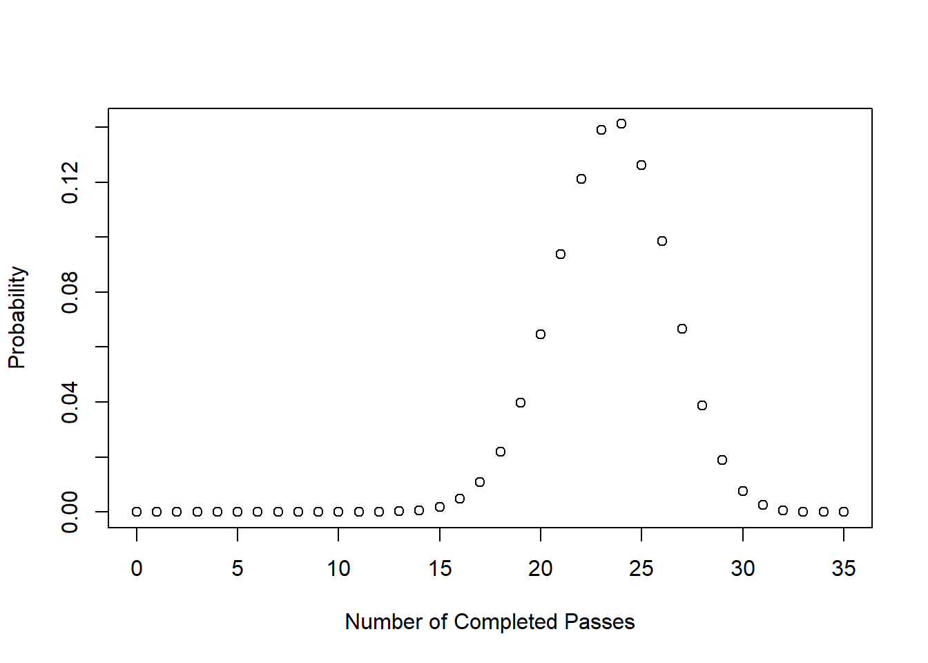
#Via Simulation

#Generate a vector to sample from the comes up 1 67% of the time and 0 33% of the time:
mahomes <- c(rep(1,67), rep(0,33))
result <- rep(NA, length(mahomes))

for(i in 1:length(result)){
  result[i] <- sum(sample(mahomes, 35, replace=T))
}

hist(result, xlim=c(0,35), ylim=c(0,0.15),freq=F )
points(0:35, probs, style="b", col="darkblue", pch=16)
#> Warning in plot.xy(xy.coords(x, y), type = type, ...):
#> "style" is not a graphical parameter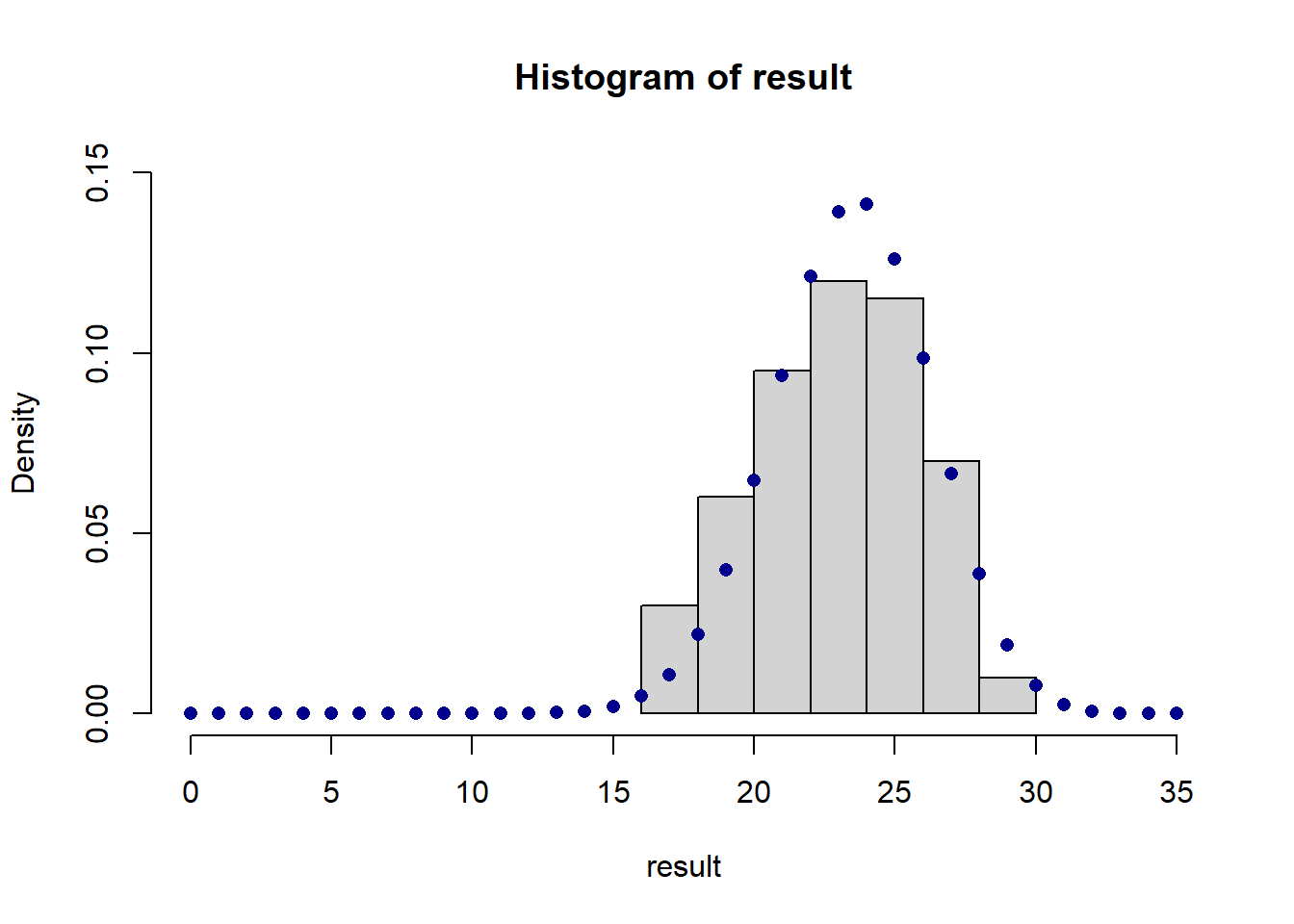
4.2 Formally Defining a RV
Why is this binomial formula helpful? First: it’s helpful to answer the sort of questions we asked above: If we see a number of successes in a given number of trials, whats the likelihood of that occurring under various probabilities? So, for example, what’s the probability of Punxsutawney Phil making a correct forecast in 7 out of the last 10 years if he is just guessing at random? We can use the information generated here to try to understand that. Indeed, this will become a very easy question to answer at the end of today’s class and next week.
But we can also think about this problem in reverse: what are some potential outcomes of the Mahomes’ performance in the superbowl, given that he is expected to complete 67% of passes?
Mahomes throws around 35 passes a game, so let’s use our formula to calculate the probability of him completing 1,2,3,4,5…35 passes.
To do so, I’m going to use the function I wrote in R last class. I’m going to determine the probability of each of these options, and then graph the result.
prob.k <- function(n,k,p){
  choose(n,k)*p^(k) * (1-p)^(n-k)
}

#Test:
3/8 ==prob.k(3,2,.5)
#> [1] TRUE

#For the first


prob.k(35,0,.67)
#> [1] 1.406008e-17
#Very unlikely!

#Give a whole vector of ks

probs <- prob.k(35, seq(0,35,1), .67)
probs
#>  [1] 1.406008e-17 9.991180e-16 3.448471e-14 7.701585e-13
#>  [5] 1.250924e-11 1.574648e-10 1.598506e-09 1.344545e-08
#>  [9] 9.554416e-08 5.819508e-07 3.071995e-06 1.417518e-05
#> [13] 5.755983e-05 2.067592e-04 6.596603e-04 1.875034e-03
#> [17] 4.758610e-03 1.079806e-02 2.192333e-02 3.982564e-02
#> [21] 6.468649e-02 9.380941e-02 1.212028e-01 1.390878e-01
#> [25] 1.411952e-01 1.261344e-01 9.849653e-02 6.665927e-02
#> [29] 3.866815e-02 1.895022e-02 7.694938e-03 2.519848e-03
#> [33] 6.395068e-04 1.180357e-04 1.409695e-05 8.177454e-07

#Display together
cbind(seq(0,35,1), probs )
#>                 probs
#>  [1,]  0 1.406008e-17
#>  [2,]  1 9.991180e-16
#>  [3,]  2 3.448471e-14
#>  [4,]  3 7.701585e-13
#>  [5,]  4 1.250924e-11
#>  [6,]  5 1.574648e-10
#>  [7,]  6 1.598506e-09
#>  [8,]  7 1.344545e-08
#>  [9,]  8 9.554416e-08
#> [10,]  9 5.819508e-07
#> [11,] 10 3.071995e-06
#> [12,] 11 1.417518e-05
#> [13,] 12 5.755983e-05
#> [14,] 13 2.067592e-04
#> [15,] 14 6.596603e-04
#> [16,] 15 1.875034e-03
#> [17,] 16 4.758610e-03
#> [18,] 17 1.079806e-02
#> [19,] 18 2.192333e-02
#> [20,] 19 3.982564e-02
#> [21,] 20 6.468649e-02
#> [22,] 21 9.380941e-02
#> [23,] 22 1.212028e-01
#> [24,] 23 1.390878e-01
#> [25,] 24 1.411952e-01
#> [26,] 25 1.261344e-01
#> [27,] 26 9.849653e-02
#> [28,] 27 6.665927e-02
#> [29,] 28 3.866815e-02
#> [30,] 29 1.895022e-02
#> [31,] 30 7.694938e-03
#> [32,] 31 2.519848e-03
#> [33,] 32 6.395068e-04
#> [34,] 33 1.180357e-04
#> [35,] 34 1.409695e-05
#> [36,] 35 8.177454e-07

#Graph to make this clearer

plot(seq(0,35,1), probs, pch=16,
xlab="Catches",
ylab="Probability of Making This Many Catches")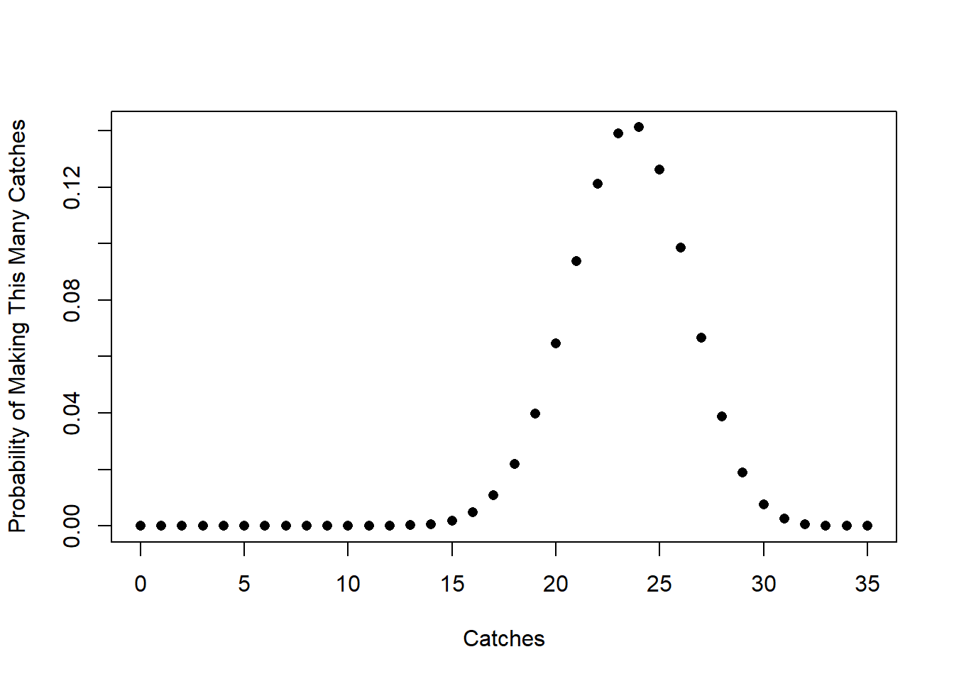
This is a description of the long term probability of what might happen, but we can also think about this as a “population” this is the function that describes the “truth” about a QB like Mahomes.
Back in week 1 I mentioned that an alternative way to define a population is as a “Data Generating Function”. This is, effectively, what we have here. If we think about what is going to happen when Mahomes plays a football game, the data is generated by this function. Each time he plays a game and throws 35 passes, we get a draw from this distribution.
Think about it like this. Let’s generate 30 games worth of data that is drawn from this binomial function, and compare it against the “truth”
Let’s first determine how to draw from this distribution. We will get to the “real” way to do this in one minute, but to be explicit we can think about drawing from the number of completions 0 to 35, with each number being pulled with the probability we calculated above. We could do this via the sample(), as it has an option prob which lets us input the probability each entry should be sampled with. Here is for one game:
So in this first game Mahomes made 25 of 35 passes.
We can shortcut this substantially, because critically, R knows the binomial function.
Because R knows what the binomial function looks like, and we can randomly generate draws from that distribution using the rbinom command, which takes as it’s argument the number of trials we are interested in, the number of attempts in each trial, and the probability:
set.seed(19104)

thirty.games <- rbinom(30,35,.67)
thirty.games
#>  [1] 25 23 23 24 22 27 22 25 24 23 26 27 24 22 24 18 22 19
#> [19] 27 28 24 26 23 19 25 21 22 22 21 27
Each of these 30 numbers is a “game”, and the number is the number of successful passes out of 30 Mahomes completed.
Let’s visualize what this looks like against the known binomial distribution for these paramaters:
selection <- sort(unique(thirty.games))
probs.selection <- prop.table(table(thirty.games))
plot(seq(0,35,1), probs, pch=16,
xlab="Catches",
ylab="Probability of Making This Many Catches", ylim=c(0,.2))
points(selection ,probs.selection, pch=16, col="firebrick")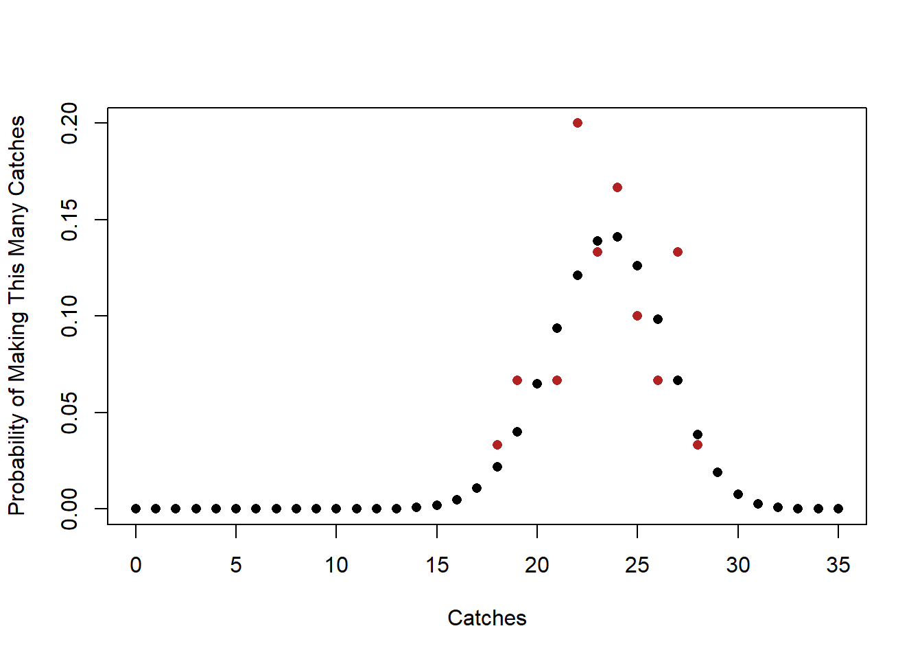
Clearly the red dots and black dots are related, but they are not exactly the same thing. The black dots are what we expect to happen in expectation or if an infinite number of football games are played. The red dots are the result of 30 realizations of that data generating process in practice.
This is what we mean when we define \(K\) as a “random variable” that is binomally distributed with n=35 and \(\pi\)=.67, where \(\pi\) is the probability of success.
When we talk about “random variables” this is a different thing than the variables in a dataset (which are samples of data). When we talk about random variables we are talking about population level distributions that produce sample of data, with each of those samples being a little bit different, yet following the same underlying truth.
Why do we need these?
In short, Random Variables are helpful because they allow us to compare a sample of data to the theoretical truth of what should happen. In other words, we can compare a sample of data to the population.
Formally, a random variable assigns a number and a probability to each event. Because we are defining events with a number and a probability, this allows us to do math! Which is good!
For example a coin flip can be represented by a binary random variable where 0 is tails and 1 is heads. This particular type of random variable is called a Bernoulli Random Variable.
For a fair coin a Bernoulli random variable \(C\) can be defined as the following:
\[ f(x) = P(C=c) = \begin{cases} .5 \text{ if } 0 \\ .5 \text{ if } 1 \end{cases} \]
We use capital letters to describe the whole random variable, and lower case letters to describe particular instances of that random variable. So we could write \(P(C=1)=.5\).
The values a random variable take on must represent mutually exclusive AND exhaustive events. Different values cannot represent the same event and all events should be represented by some variables. If I defined a random variable that described the probability people were of different races in a sample of data, I couldn’t have 1=White, and 2=White or Black (not mutually exclusive). I also couldn’t have a random variable for race what was only 1=White, 2=Black, 3=Asian, because that’s not exhaustive.
Anything that has these values can be defined as a Random Variable. However, there are several “standard” random variables that take on distributions with known properties that we frequently use and refer to in statistics. The Bernoulli RV is one, as is the Binomial RV (last time, and to come).
There are two types of random variables: discrete and continuous. Discrete RVs take a finite number of values. The Bernoulli RV above is discrete because it can take on a finite number of values. A continuous RV which can take on any real value within a given interval. Examples of a continuous RV are height, weight, or GDP. (We will cover these next week).
The above example of a Bernoulli RV allows us to think more about the nature of RVs. The math array we saw above, which described the values that the RV can take on and the probability that each of those values occur, is called the Probability Mass Function(PMF).
We can graph the PMF for the above Bernoulli RV (though it won’t be very interesting).
#Bernoulli RV PMF

plot(c(0,1), c(.5,.5), pch=16, xlim=c(-1,2))
segments(0,0,0,.5)
segments(1,0,1,.5)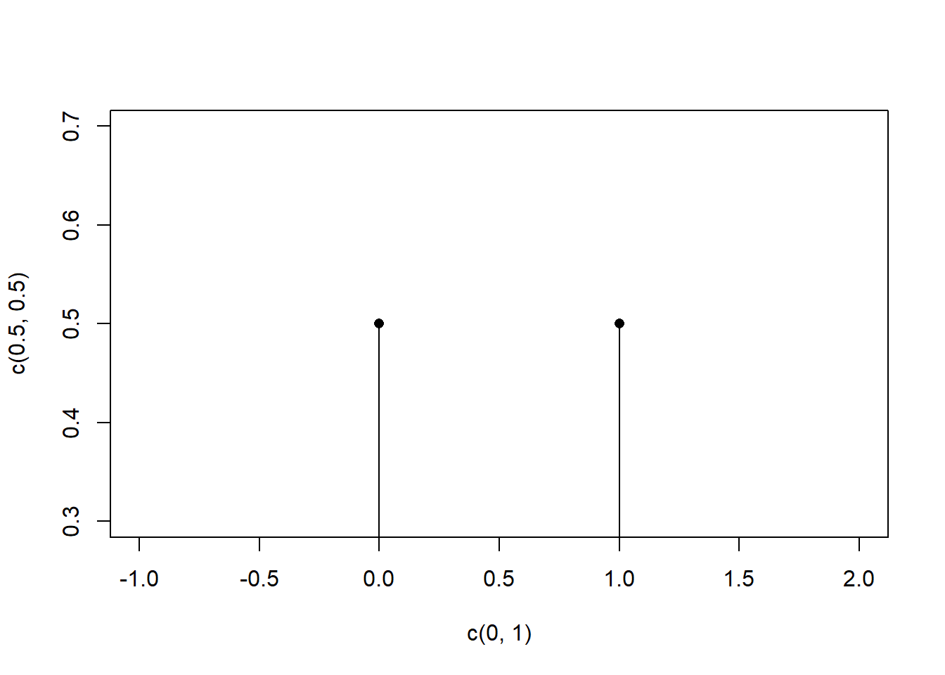
Another important function related to the probability distribution is the cumulative distribution function. The CDF of a random variable represents the cumulative probability that a random variable take a value equal to or less than a specific value.
Another way to think about this is that the CDF is the sum of the PMF for all values less than or equal to the value of interest.
Formally:
\[ CDF = F(x) = P(X \leq x) = \sum_{k < x} f(x) \]
The CDF of a Bernoulli RV is extremely straight forward. For all values of X we simply add up the probability to the left in the PMF:
#Drawing a Bernoulli RV CDF

plot(c(0,1), c(0,.5), ylim=c(0,1), xlim=c(-1,2))
points(c(0,1), c(.5,1), pch=16)
segments(-5,0,0,0)
segments(0,.5,1,.5)
segments(1,1,5,1)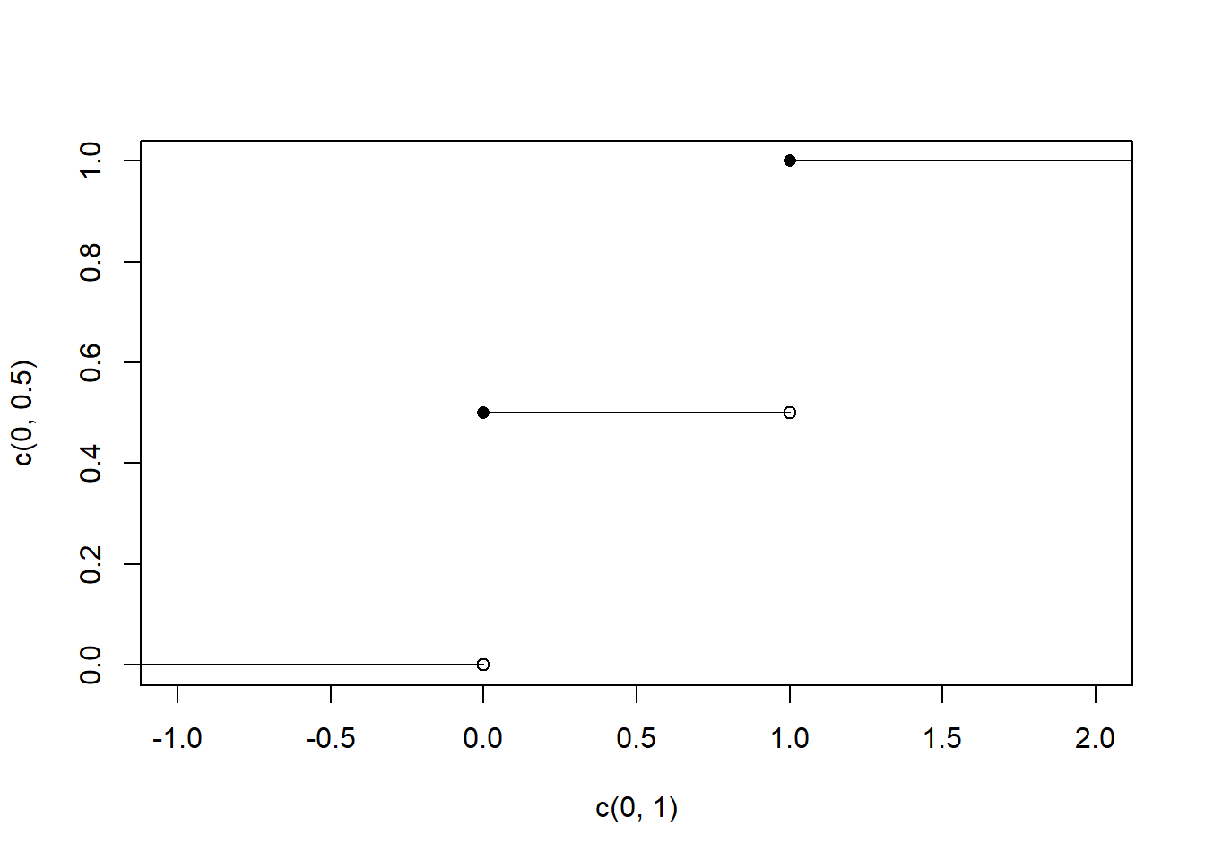
The CDF, by definition, approaches 0 as the variable gets closer to negative infinity, and approaches 1 as the variable gets closer to positive infinity. The CDF can never decrease as the variable increases.
The two distributions: the PMF and CDF are 1:1 related. If you give me the PMF I’ll give you the CDF. If you give me the CDF i’ll give you the PMF.
(Draw these as well)
For example if a PMF is
\[ f(x) = P(C=c) = \begin{cases} .1 \text{ if } 0 \\ .25 \text{ if } 1 \\ .5 \text{ if } 2 \\ .15 \text { if } 3 \\ \end{cases} \]
Then the corresponding CDF would be:
\[ F(x) = P(C \leq c) = \begin{cases} 0 \text{ if } c \leq 0\\ .1 \text{ if } 0 \leq c< 1 \\ .35 \text{ if } 1 \leq c <2 \\ .85 \text{ if } 2 \leq c < 3 \\ 1 \text { if } 3 \leq c \\ \end{cases} \]
Or if I defined a CDF as:
\[ F(x) = P(C \leq c) = \begin{cases} 0 \text{ if } c<-2\\ \frac{1}{5} \text{ if } -2 \leq c < 1.5 \\ \frac{3}{5} \text{ if } 1.5 \leq c <3 \\ \frac{4}{5} \text{ if } 3 \leq c < 5 \\ 1 \text { if } 5 \leq c \\ \end{cases} \]
What is the corresponding PMF?
\[ f(x) = P(C=c) = \begin{cases} \frac{1}{5} \text{ if } -2 \\ \frac{2}{5} \text{ if } 1.5 \\ \frac{1}{5} \text{ if } 3 \\ \frac{1}{5} \text { if } 5 \\ \end{cases} \]
The Binomial Random Variable is what we defined last class, and describes the distribution of a sequence of i.i.d. (\(k\)) Bernoulli trials.
This term “i.i.d.” is going to come up a lot. What do we mean by independent and identically distributed.
We’ve seen that a sequence of 3 coin flips is a binomial random variable, so something like \(\lbrace H H T \rbrace\), is a realization of this RV. These three events are all independent from one another: getting a Head on the first flip doesn’t change the probability on the second flip. These three flips are identically distributed because each has the same probability (say, 50%, though it doesn’t need to be) of being selected. We can also think of a roulette wheel as an example of iid. Each roll of the roulette wheel is independent from the one previous (despite casino’s displaying the previous outcomes!), and each time the wheel spins the same numbers are in play. A random sample survey is also IID. Me getting selected doesn’t impact the probability of anyone else getting selected, and each time we make a selection it’s from the same pool of people.
We have also already seen what the PMF of a binomial random variable looks like. For example the PMF for a Binomial with 3 trials and a probability of success of .5 looks like:
\[ f(K) = p(K=k) = \begin{cases} \frac{1}{8} \text{ if } 0\\ \frac{3}{8} \text{ if } 1\\ \frac{3}{8} \text{ if } 2\\ \frac{1}{8} \text{ if } 3 \end{cases} \]
What would the CDF of this RV look like?
\[ F(k) = P(K \leq k) = \begin{cases} 0 \text{ if } k< 0 \\ \frac{1}{8} \text{ if } 0 \leq k < 1\\ \frac{1}{2} \text{ if } 1 \leq k < 2\\ \frac{7}{8} \text{ if } 2 \leq k < 3\\ 1 \text{ if } 3 \leq k \\ \end{cases} \]
Given that the binomial distribution is a known distribution, it makes sense that R knows what the shape of it is and can draw it.
To get the PMF of a binomial random variable we can use the dbinom() command. Looking at the help file, this command wants x a vector of quantaties, size the number of trials, and prob the probability of success and failure. The only thing that’s a little bit confusing here is x: but that’s just telling us for what values of the pmf we want probabilities for.
So for example, if I want the full PMF for the binomial random variable with 10 trials with a probability of success of .3:
dbinom(x=0:10, size=10, prob=.3)
#>  [1] 0.0282475249 0.1210608210 0.2334744405 0.2668279320
#>  [5] 0.2001209490 0.1029193452 0.0367569090 0.0090016920
#>  [9] 0.0014467005 0.0001377810 0.0000059049
Plotting these is as easy as plotting the probabilities next to the numbers they represent:
probs <- dbinom(x=0:10, size=10, prob=.3)
plot(0:10, probs, xlab="Number of Successes", ylab="P(X=x)", pch=16,
     main="PMF for n=10 p=.3")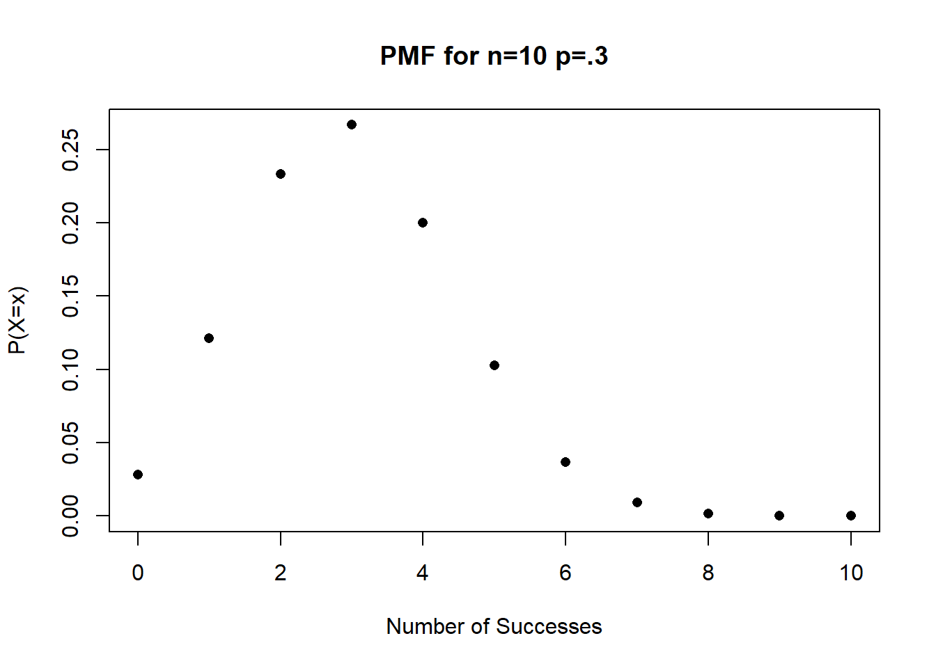
What about the CDF? We could imagine using the output of dbinom() to calculate the CDF, but we don’t actually have to. R has a build in function pbinom() to calculate the CDF.
pbinom(0:10, 10, .3)
#>  [1] 0.02824752 0.14930835 0.38278279 0.64961072 0.84973167
#>  [6] 0.95265101 0.98940792 0.99840961 0.99985631 0.99999410
#> [11] 1.00000000
This lines up well with what we know about the CDF. I can visually see that the first entry in the PMF and CDF functions are equal, and that the second entry in the CDF output is the first two in the PMF output added together.
Again, this is easy to graph:
probs <- pbinom(0:10, 10, .3)
plot(0:10, probs, xlab="Number of Successes",
     ylab="P(X <= x)", main="CDF for n=10 p=.3", pch=16)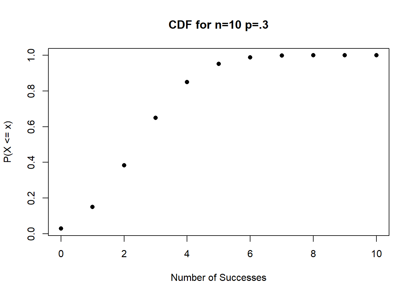
Note that these function are smart(ish, and will give you warnings for impossible answers:
dbinom(0.5, 10, .3)
#> Warning in dbinom(0.5, 10, 0.3): non-integer x = 0.500000
#> [1] 0
This is looking ahead to next week, but think about the kind of cool questions can be answered using that pbinom() function. If Jalen Hurts throws 35 passes in the Superbowl this weekend, what is the probability he completes at least 25 given his season completion rate of 66.5%?
The pbinom() function can give us the cumulative probability that Hurts throws 24 passes or fewer:
pbinom(24, 35, .665)
#> [1] 0.6633012
So the probability of throwing 25 passes or greater is 1-.66 = 34%.
4.3 Expectation and Variance
We have just seen that if you give R two pieces of information (the number of trials and the probability of success) it can give you an exact PMF and CDF.
That’s great, but we need to have some ability to describe the shape of these distributions.
For sample level variables we have seen before that two key measurements are the mean and the standard deviation. The mean is a measure of central tendency, and the standard deviation is a measure of the dispersion. Together those give a good sense of what is happening in a sample.
At the level of distributions/populations the equivalent measures are the expected value and the variance.
Again: these things do not apply to samples of data, they are ways to talk about populations/distributions.
The expected value is the average value of the RV we would get if we sampled a large number of times.
If a Bernoulli random variable takes on two values: 0 for tails (failure), and 1 for success (heads), and the probability of success (\(\pi\)) is .5, what is the expected value?
We expect there to (eventually) be approximately the same number of 0s and 1s, so the expected value will be .5.
More formally: the expected value of any random variable is equal to the sum of each realization multiplied by the probability of that realization.
Formally: \(E[X] = \sum_x xp(x)\)
For a Bernoulli Random Variable this would be: \(E[X] = 0*(1-\pi) + 1*\pi = \pi\). The expected value for a Bernoulli random variable is just the probability of success. (That makes sense!).
What about for a Binomial random variable? There the RV can take on any value from 0 to \(n\). So the expected value equals:
\[ \begin{align} E[X] = &\sum_x xp(x) \\ = &0*p(X=0) + 1*p(X=1) + 2*p(X=2) + \dots + n*p(X=n) \end{align} \]
So for this Binomial RV for n=3 and \(\pi = .5\)
\[ f(K) = p(K=k) = \begin{cases} \frac{1}{8} \text{ if } 0\\ \frac{3}{8} \text{ if } 1\\ \frac{3}{8} \text{ if } 2\\ \frac{1}{8} \text{ if } 3 \end{cases} \]
The expected value is:
\[ \begin{align} E[X] = &\sum_x xp(x) \\ = &0*\frac{1}{8} + 1*\frac{3}{8} + 2*\frac{3}{8} + 3*\frac{1}{8}\\ = 1.5 \end{align} \]
There is, however, a shortcut for the expected value of binomial RVs based on the fact that they are made up of \(n\) Bernoulli random variables by definition. Because the expected value of each Bernoulli draw is \(\pi\) and the number of Bernoulli RVs is \(n\). The expected value of a Binomial RV can also be given by \(E[X] = n\pi\).
For the above example: \(E[X] = n\pi=3*.5=1.5\).
The second important way to measure a random variable is through its variance, a measure of how spread out the distribution is.
The variance of a random variable X is defined by \(V[X] = E[(X-E(X))^2]\). If we think about this, what this is saying is the variance is the expected (squared) deviation from the overall expected value.
The textbook discusses how another (slightly easier math) way of thinking about the variance is to express it as \(V[X] = E(X^2) - E(X)^2\)
From that, if we consider a Bernoulli RV where \(E[x] = \pi=.5\). Then the variance is equal to:
\[ \begin{align} V[X] = &E(X^2) - E(X)^2\\ = & E(X)^* - E(X)^2\\ = & \pi - \pi^2\\ = &\pi(1-\pi)\\ \\ &\text{*Because: } 1^2=1 \text{ and } 0^2=0 \end{align} \]
This is a neat result (neat to me), that says that the variance of a Bernoulli variable increases as you get closer to 50/50. Indeed, we can graph what the expected variance of a Bernoulli RV is for all levels of \(\pi\)
pi <- seq(0,1,.001)
plot(pi, pi*(1-pi), type="l", xlab="pi", ylab="Variance",
     main="Variance of Bernoulli RV")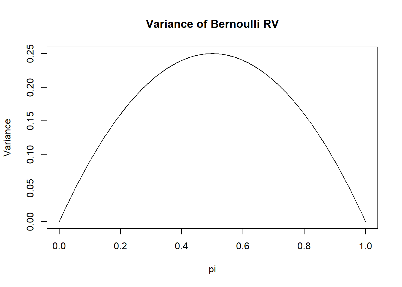
Impportantly, the variance can never be negative because it’s squared. But also theoretically it’s not clear what that would mean. We can take the square root of the variance to get the population level standard deviation. Again, this is different then the sample standard deviation. We will frequently represent the population variance as \(\sigma^2\) and the population standard deviation as \(\sigma\)
What is the variance of our working example binomial distribution?
\[ f(K) = p(K=k) = \begin{cases} \frac{1}{8} \text{ if } 0\\ \frac{3}{8} \text{ if } 1\\ \frac{3}{8} \text{ if } 2\\ \frac{1}{8} \text{ if } 3 \end{cases} \]
We can apply the variance formula:
\[ \begin{align} E[K^2] = &0*\frac{1}{8} + 1*\frac{3}{8} + 4*\frac{3}{8} + 9*\frac{1}{8} = &\frac{3}{8}+\frac{12}{8} + \frac{9}{8} = \frac{24}{8} = 3\\ E[K] = &(n\pi)^2 = (3*.5)^2 = 1.5^2 = 2.25\\ V[K] = &E[K^2] - E[K]^2\\ = &3-2.25 \\ = &.75 \end{align} \]
That’s a lot to calculate! But again, just thinking of this as the sum of \(n\) i.i.d Bernoulli trials, the variance of a Binomial simplifies down to \(V[X] = np(1-p)\).
As such, the variance of the above Binomial RV is: \(V[X] = np(1-p) = 3*.5*(1-.5)=.75\).
The variance of binomial similarly is largest when \(\pi=.5\), and scales linearly for however may trials you are interested in.
Here is what I’d like for you to think about in R for the remainder of the time:
For \(n=200\), on one graph, can you use the dbinom() function to plot the Binomial RV for \(\pi = \lbrace .1,.25,.5,.75,.9 \rbrace\)? Looking at these distributions, what does it mean for our ability to identify potential outlier situations given different underlying truths?