9 Hypothesis Tests
9.1 Review
We saw last week that if we have a sample of data and do not know the population (which we usually do not), then we can still estimate a sampling distribution by subbing in the the sample variance.
Specifically we claimed that:
\[ \frac{\bar{X_n}-E[X]}{s/\sqrt{n}} \sim t_{n-1} \]
The sampling distribution of the sampling mean is \(t\) distributed with \(n-1\) degrees of freedom.
We were able to use that information to generate a confidence interval around a sample mean using this formula:
\[CI(\alpha) = [\bar{X_n}-t_{\alpha/2}*SE,\bar{X_n}+t_{\alpha/2}*SE]\]
Where \(\alpha\) is the inverse proportion of our confidence level.
So if I had a sample of \(n=8\) with \(\bar{x}=4\) and \(s=2\), then the 90% confidence interval would be:
#Calculate t score for alpha=.05
t <- qt(.05,df=7)*-1

#SE
se <- 2/sqrt(8)

#Confidence interval
c(4-t*se,4+t*se)
#> [1] 2.660331 5.339669
There is a 90% chance the true population parameter is between these two values. OR 90% of similarly constructed confidence intervals will contain the true population parameter.
When we have a sample and know nothing about the population it shifts the types of questions we want to ask. Again, on the midterm (and on Q1 of the problem set this week), we are asking a question like: if the truth is X and we take a sample of size \(n\) what is likely to happen? When we don’t know the truth, instead we have to ask questions like: what is plausible or likely to be true? We now have one method to determine this: confidence intervals. A confidence interval gives us a range which contains the truth with some probability (If we are being loose with the definition).
9.2 The logic of hypothesis testing
The second method which we can use to determine a plausible value for the truth is via a hypothesis test.
Let’s return to the example of me in October 2022 trying to predict what will happen in the election using polls. In hindsight we know the true level of support for candidates that would generate these polls, but I didn’t at the time.
Here is a (fake) poll of 1000 people in Pennsylvania:
set.seed(19102)
pa.poll <- rbinom(1000,1, .525)
mean(pa.poll)
#> [1] 0.53
var(pa.poll)
#> [1] 0.2493493
sd(pa.poll)
#> [1] 0.4993489
This would be all the information I have about this poll.
Now we have learned how to put a 95% confidence interval around this value, and as a pollster I often will do that:
qt(.025, df=999)
#> [1] -1.962341
se <- sd(pa.poll)/sqrt(1000)

#Confidence Interval
c(mean(pa.poll)-1.96*se ,mean(pa.poll)+1.96*se)
#> [1] 0.49905 0.56095
So there is a 95% chance the true level of support for Fetterman is between 49.9% and 56.1%. Not particularly re-assuring.
That’s helpful for public consumption, but what if Kornacki comes to me and says “Hey Marc, I know your poll has Fetterman ahead, but can you actually say with certainty that Fetterman is going to win? Could the race be tied instead?” (Kornacki does not actually talk to me).
How can we answer this question?
What, right now, do we know about the sampling distribution of the proportion of voters who support Fetterman? Do we know where it is centered? Nope. Definitely not. We have one sample mean out of many possible. We feel like the truth is probably in the the 50% range, but can’t say much more than that.
Do we know how wide the sampling distribution is? Yes! We definitely do.
The CLT says that the sampling distribution will be \(\bar{X_n} ~ N(\mu=E[X], \sigma^2=V[X]/n]\). We don’t know \(E[X]\), but we have seen that the sample variance of X is a reasonable stand-in for \(V[X]\). Technically when we use the sample variance the sampling distribution is t distributed, but we also know that with sufficiently large samples the t distribution is equal to the standard normal. So in this case i’m pretty confident in saying that the sampling distribution of Fetterman support is \(\bar{X_n} \sim N(\mu=E[X], \sigma^2=.249/1000]\).
Ok so we know that what the width of this normal distribution is, why does that help us?
It helps us because we can make an inference via contradiction (the fancy way to say this). Let’s think about the question that Kornacki asked us: can we rule out that the race is tied in favor of the idea that Fetterman is winning? In other words, if the race was tied, would it be particularly special or crazy to get this result? If that’s the question we want to answer, we can posit: if the truth was 50%, would it be special to get a mean of 53%? If we deem that it is crazy or special than we can reject the idea that the race is tied.
So, let’s posit that support for Fetterman is \(\bar{X_n} ~ N(\mu=.5, \sigma^2=.249/1000]\). What would that look like?
eval <- seq(.45,.55, .0001)
plot(eval, dnorm(eval, mean=.5, sd=sqrt(.249/1000)), type="l",
     main="Sampling Distribution of Fetterman Support: Tied Race")
abline(v=.5,lty=2)
abline(v=mean(pa.poll), lty=2, col="firebrick")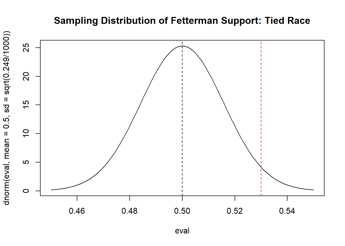
If the race was tied we believe that this would be the distribution that produces means. If this is the case, what is the probability that we get exactly 53% as the result? Trick question! It’s 0. Instead, we are going to ask: what is the probability we get something as extreme of more extreme than 53%? In other words, what is the probability to the right of the red line in the above figure?
Around 2.86%, so pretty low! In this case, with these specific data, I would reject the idea that this race is tied.
To be clear, what we are saying here is: if the truth is that the race is tied, 2.86% of means will be equal to or greater than what we got in our sample.
But let’s be a bit more principled about this: let’s say that we will reject the idea that the race is tied for the idea that Fetterman is leading if there is less than 5% chance of seeing something as extreme or more extreme than what we get in our sample.
In other words: we would reject the idea the race is tied for the idea that Fetterman is leading if the sample mean is to the right of this blue line:
eval <- seq(.40,.60, .0001)
plot(eval, dnorm(eval, mean=.5, sd=sqrt(.249/1000)), type="l",
     main="Sampling Distribution of Fetterman Support: Tied Race", xlab="Support",
     ylab="Density")
abline(v=.5,lty=2)
abline(v=mean(pa.poll), lty=3, col="firebrick")
abline(v=qnorm(.05, mean=.5, sd=sqrt(.249/1000), lower.tail = F ),
       col="darkblue", lty=2)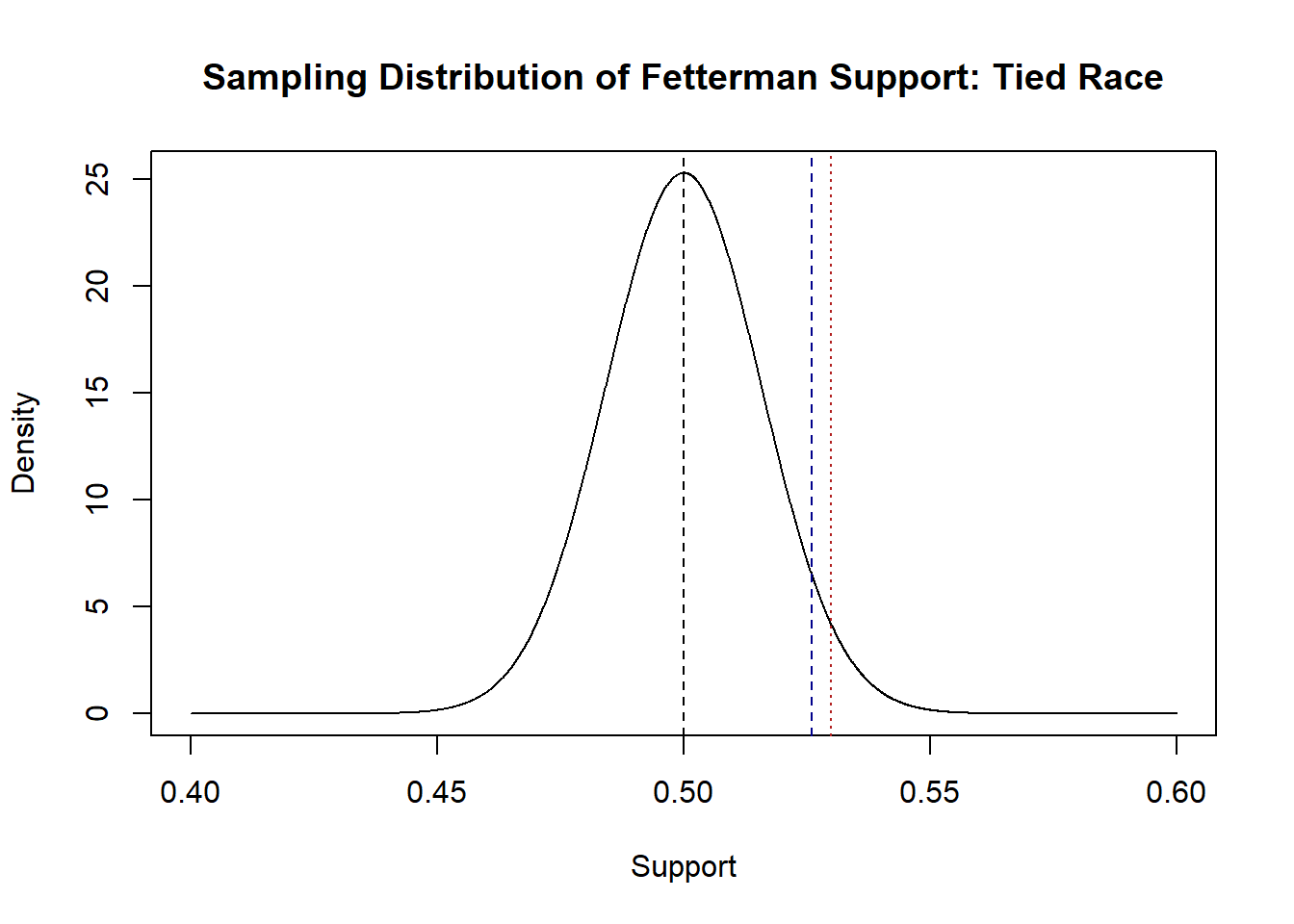
To reiterate this, what we are setting up is a zone where, if the truth was that the race was tied and this distribution was generating means, there is less than a 5% chance that a mean would be produced that was to the right of that blue line.
In this particular case we would reject the idea that the race is tied, because the sample mean is greater than the blue line, meaning there is a less than 5% chance that this mean would be produced if the truth was that the race was tied. Importantly: remember that we know the truth here and the race is not tied, Fetterman is going to win this race! So, in this case we have made the correct inference about the population.
OK: we now have a method for a single sample to determine the relatively likelihood of a certain population value being true given the mean we actually get in our sample.
We call the 5% level here \(\alpha\) (yes, it’s the same \(\alpha\) as last time which will get to shortly), which is the probability of mistakenly concluding that Fetterman is leading if the race is actually tied. This is a false positive: we think there is something there when there actually is not.
In the case so far we were interested in finding out if the race was tied or if Fetterman was leading. Another more conservative possibility is to consider whether or not the race is tied, and be agnostic about who is leading the race.
In this case we can consider our original sampling distribuion, again centered around 50% (the tie). Again, we want to set up a zone where there is a 5% we will see something that extreme if the truth is 50%. Because now we are agnostic about who is winning the race, we need to put this in both tails. And because we want for this to represent a zone that has, in total, a 5% chance of occurring, we will put 2.5% in each tail.
eval <- seq(.45,.55, .0001)
plot(eval, dnorm(eval, mean=.5, sd=sqrt(.249/1000)), type="l",
     main="Sampling Distribution of Fetterman Support: Tied Race")
abline(v=.5,lty=2)
abline(v=mean(pa.poll), lty=2, col="firebrick")
abline(v=qnorm(.025, mean=.5, sd=sqrt(.249/1000)), col="darkblue", lty=2)
abline(v=qnorm(.025, mean=.5, sd=sqrt(.249/1000), lower.tail = F), col="darkblue", lty=2)
We have specifically set a zone where, if the race is tied, than there is a 5% chance of drawing a mean. If our mean is within that zone, then there is less than a 5% chance of it occurring by chance under the null hypothesis.
In this case our mean actually lies outside of this zone. As such, we cannot reject the idea that the race is tied as a sampling distribution centered around a tie would produce a mean at least this extreme a rate that is greater than 5%. Put into regular language: we cannot rule out with our stated level of confidence that the race is not tied.
Unsurprisingly, given the way that we set up these tests and the fact that our sample mean of 53% didn’t change, this test (what we will call a two-tailed test) is more conservative. It’s harder for any given mean to be in the rejection zone for a two tailed test.
To recap: because we can draw the shape of the sampling distribution given the information contained in one sample, we can ask the question: if \(E[X]\) was 50% ( and really we could put any value in here), what is the probability of getting the result that we did? Is that probability less than 5%? If so, we are happy with the possibility of a false positive, and will reject the idea that the race is tied.
9.3 Formalizing a hypothesis test.
The above should have given you the basic intuition for a hypothesis test. Now we will formalize the steps of a hypothesis test.
Here are the steps, which we will go through one at a time. These are the same steps that are in your textbook.
- Specify a null hypothesis and an alternative hypothesis.
- Choose a test statistic and the level of test (\(\alpha\)).
- Derive the sampling distribution and center on the null hypothesis.
- Compute the p-value (one sided or two sided).
- Reject the null hypothesis if the p-value is less than or equal to \(\alpha\). Otherwise retain the null hypothesis.
- First is specifying the null and alternative hypotheses. The null hypothesis is the thing that we are looking to contradict with our test. Above, our null hypothesis was that the race was tied (proportion voting Fetterman was .5). But the null hypothesis can be anything. For example we could be sampling incomes and may want to know if our sample has an income that is significantly different from the mean income in the United States. In that case the mean income of the United States would be our null hypothesis. We specify the null hypothesis as \(H_0\). In the Fetterman case above we would specify the null hypothesis as:
\(H_0: P(Fetterman)=.5\)
When we get to the alternative hypothesis we have our first decision to make. Above we looked at two different things: first we testing whether the race was tied against whether Fetterman was leading. In that case we would set our alternative hypothesis to be that Fettermans support is greater than the null hypothesis:
\(H_a: P(Fetterman)>.5\)
In this case we only reject the null hypothesis if we have evidence that the truth is greater than the null hypothesis. We call this a “One tailed test”.
The second things we tested is whether the race was tied or not. Here we are agnostic about whether our sample mean is extremely above or below the null hypothesis. We would specify this alternative hypothesis as:
\(H_a: P(Fetterman) \neq .5\)
We call this a “Two-tailed test”.
- The test statistic is simply the thing we are hypothesis testing. In this case it is the sample mean: 53%. The \(\alpha\), as we discussed, is the probability of a false positive we are comfortable with. This is the false positive rate because by random chance 5% of the sample means will be in this zone if the null hypothesis is true. This \(\alpha\) can be anything, but 5% is a pretty standard number.
Derive the sampling distribution and center on the null hypothesis. To calculate the sampling distribution all we need to know is the standard error. We calculated this above for our sample, but note here that nothing about these steps refer to the sample mean specifically: anything with a known sampling distribution can make use of these steps!
Compute the p-value. This step is slightly different than what we did above, but uses the exact same logic. What we want to calculate is the probability of getting something as extreme or more extreme than our test statistic if the null hypothesis is true.
The important thing here is that the calculation of the p-value changes based on whether we are doing a one-tailed or two-tailed test.
For a one tail test the p-value is the area in the tail more extreme than our test statistic in the direction of the test.
Above we were testing the alternative hypothesis that Fetterman’s support was greater than .5:
eval <- seq(.40,.60, .0001)
plot(eval, dnorm(eval, mean=.5, sd=sqrt(.249/1000)), type="l",
     main="Sampling Distribution of Fetterman Support: Tied Race", xlab="Support",
     ylab="Density")
abline(v=.5,lty=2)
abline(v=mean(pa.poll), lty=3, col="firebrick")
Here the p value would be:
The probability of seeing a result this extreme if the null was true is 2.86%.
If we doing a two-tailed test we have to account that we are agnostic about whether the truth might be greater or less than the null. Because of this, we test to see the probability of getting a value as extreme or more extreme in both directions. Visually, we test to see the total probability of getting something in the tails to the left or right of our test statistic, and our test statistic flipped to the other side of the mean:
eval <- seq(.40,.60, .0001)
plot(eval, dnorm(eval, mean=.5, sd=sqrt(.249/1000)), type="l",
     main="Sampling Distribution of Fetterman Support: Tied Race", xlab="Support",
     ylab="Density")
abline(v=.5,lty=2)
abline(v=mean(pa.poll), lty=3, col="firebrick")
abline(v=.5 - (mean(pa.poll)-.5), lty=3, col="firebrick")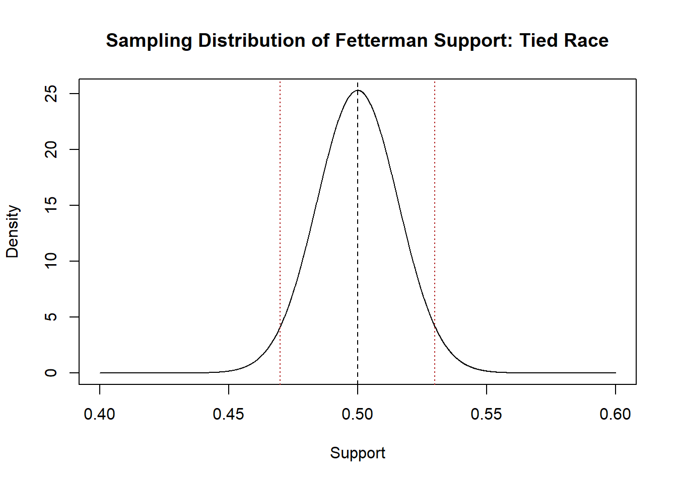
So adding up the probability in each of those tails:
pnorm(mean(pa.poll), mean=.5, sd=sqrt(.249/1000), lower.tail=F) + pnorm(.5 - (mean(pa.poll)-.5), mean=.5, sd=sqrt(.249/1000), lower.tail=T)
#> [1] 0.05727939
There is a 5.7% chance of seeing a result this extreme or more extreme if the null is true.
Note, however, that we didn’t really need to calculate that second pnorm. The normal distribution is symmetrical around the mean, so the probability to the right of 53% is exactly equal to the probability to the left of 47%. So we can do:
Said shorter: the two-tailed p-value is the one-tailed p-value doubled.
- Reject the null hypothesis if the p-value is less than or equal to \(\alpha\). Here we have set \(\alpha\) to be .05.
Therefore if we are doing a one tailed test we would reject the null hypothesis that the race is tied for the alternative hypothesis that Fetterman is leading.
However if we were doing a two-tailed test we would fail to reject the null hypothesis that the race is tied.
Notice that I did not say: we accept the null hypothesis. This is a matter of theory and taste, but to me the goal here is to set up the null hypothesis and determine if our test statistic is plausible if the null is true. That’s all we are doing. If we decide that the test statistic is plausible, it’s not really evidence that the null is true.
Before we do another example: what is the relationship between a hypothesis test and confidence intervals?
I mentioned above that our value for \(\alpha\), what we want the false positive rate to be, is the same \(\alpha\) that we used when constructing confidence intervals. As it turns out, if we construct a confidence interval with \(\alpha=.05\) and that confidence interval does not contain the null hypothesis, then a hypothesis test with \(\alpha=.05\) will also reject the null hypothesis.
So to continue our example:
#Construct a 95\% confidence interval
mean(pa.poll)
#> [1] 0.53
t.value <- qt(.025, df=999)*-1

ci <- c(mean(pa.poll)-t.value*sqrt(.429/1000), mean(pa.poll)+t.value*sqrt(.429/1000) )
library(dplyr)
#> Warning: package 'dplyr' was built under R version 4.1.3
#>
#> Attaching package: 'dplyr'
#> The following objects are masked from 'package:stats':
#>
#>     filter, lag
#> The following objects are masked from 'package:base':
#>
#>     intersect, setdiff, setequal, union
between(.5,ci[1], ci[2] )
#> [1] TRUE
#Null is within the CI

#Hypothesis test:
p <- pnorm(mean(pa.poll), mean=.5, sd=sqrt(.249/1000), lower.tail=F)*2
p>.05
#> [1] TRUE

#Let's do it a bunch of times to make sure:
reject.null.ci <- rep(NA, 10000)
reject.null.hyp <- rep(NA, 10000)

for(i in 1:10000){
  samp <- pa.poll <- rbinom(1000,1, .525)
  xbar <- mean(samp)
  se <- sqrt(sd(samp)/1000)

#ci
  ci <- c(xbar-t.value*se, xbar+t.value*se )
  reject.null.ci[i] <- between(.5, ci[1],ci[2])
#hypothesis
  p <-  pnorm(xbar, mean=.5, sd=se, lower.tail=F)*2
  reject.null.hyp[i] <- p>.05
}

table(reject.null.ci, reject.null.hyp)
#>               reject.null.hyp
#> reject.null.ci FALSE TRUE
#>          FALSE  1185    0
#>          TRUE      0 8815
#Same!
Let’s do an example with some real data:
Here is some real data for the final 2 weeks of our poll in Arizona:
library(rio)
sm.az <- import("https://github.com/marctrussler/IIS-Data/raw/main/AZFinalWeeks.csv")
head(sm.az)
#>   V1           id     weight week bi.week state county.fips
#> 1  1 118158025617 0.03165892   43      22    AZ        4013
#> 2  2 118157557679 0.89310665   43      22    AZ          NA
#> 3  3 114153878749 1.06902117   43      22    AZ          NA
#> 4  4 118159457343 0.07919169   43      22    AZ       25027
#> 5  5 118157881702 2.06085504   43      22    AZ          NA
#> 6  6 118158946302 3.62068552   43      22    AZ       36047
#>         senate.topline governor.topline      biden.approval
#> 1             Democrat         Democrat    Somewhat approve
#> 2                 <NA>             <NA>    Somewhat approve
#> 3                 <NA>             <NA> Somewhat disapprove
#> 4                 <NA>             <NA> Somewhat disapprove
#> 5 Other/Would not Vote       Republican    Somewhat approve
#> 6 Other/Would not Vote         Democrat                <NA>
#>   presvote2020         pid     ideology
#> 1          dem    Democrat     Moderate
#> 2          dem    Democrat Conservative
#> 3    dnv/other  Republican Conservative
#> 4    dnv/other Independent     Moderate
#> 5    dnv/other    Democrat      Liberal
#> 6    dnv/other  Republican     Moderate
#>   most.important.problem abortion.policy age     race
#> 1              Inflation            <NA>  37    black
#> 2       Crime and safety            <NA>  24    asian
#> 3              Inflation            <NA>  46 hispanic
#> 4              Inflation            <NA>  23    black
#> 5               Abortion            <NA>  28    black
#> 6                   <NA>            <NA>  77    white
#>   gender hispanic             education
#> 1   male    FALSE  Post graduate degree
#> 2   male     TRUE    Associate's degree
#> 3   male     TRUE      College graduate
#> 4 female    FALSE          Some college
#> 5 female    FALSE  Post graduate degree
#> 6   male    FALSE High school or G.E.D.
Let’s similarly try to determine the truth about the senate race in this state. First let’s charecterize the race in terms of the two-party vote for Democrat Mark Kelly (who actually won 52.4% of the two party vote):
table(sm.az$senate.topline)
#>
#>             Democrat Other/Would not Vote
#>                 1368                  349
#>           Republican
#>                 1245

sm.az$DemSenateVote <- NA
sm.az$DemSenateVote[sm.az$senate.topline=="Democrat"]<- 1
sm.az$DemSenateVote[sm.az$senate.topline=="Republican"]<- 0
mean(sm.az$DemSenateVote,na.rm=T)
#> [1] 0.5235362
table(sm.az$DemSenateVote)
#>
#>    0    1
#> 1245 1368
sum(table(sm.az$DemSenateVote))
#> [1] 2613
Now as it turns out this poll is almost miraculously close to the truth (this is unweighted so this is truly just a happy coincidence). But at the time I wouldn’t have known that.
Again, in this situation I have a poll that is telling me that Kelly is leading, but I know that if I took another poll of 2613 people I would get a slightly different answer every time. If I take into account how much randomness there is around sample means, would it be odd to get a sample mean of 52.4%?
Let’s go through the formal steps of the hypothesis test:
- Specify a null hypothesis and an alternative hypothesis.
The “default” for all polling and social science is to do a two-tailed test. Why? Because we like that it’s more conservative (more to come on that). So let’s set up a null and alternative hypothesis for a two-tailed test.
\[ H_o: P(Kelly)=.5\\ H_a: P(Kelly)\neq.5\\ \]
- Choose a test statistic and the level of test (\(\alpha\)).
Our test statistic is the sample mean:
mean(sm.az$DemSenateVote,na.rm=T)
#> [1] 0.5235362
And we will go with the standard \(\alpha=.05\).
- Derive the sampling distribution and center on the null hypothesis.
We believe that this sample means comes from a sampling distribution that is t distributed with 2612 degrees of freedom. In this case because the \(n\) is sufficiently large, this distribution will be well approximated by the normal distribution. As such the sampling distribution will look like:
s <- sd(sm.az$DemSenateVote,na.rm=T)

eval <- seq(.40,.60, .0001)
plot(eval, dnorm(eval, mean=.5, sd=s/sqrt(2613)), type="l",
     main="Sampling Distribution of Kelly Support: Tied Race", xlab="Support",
     ylab="Density")
abline(v=.5,lty=2)
abline(v=.524, lty=3, col="firebrick")
abline(v=.5 - (.524-.5), lty=3, col="firebrick")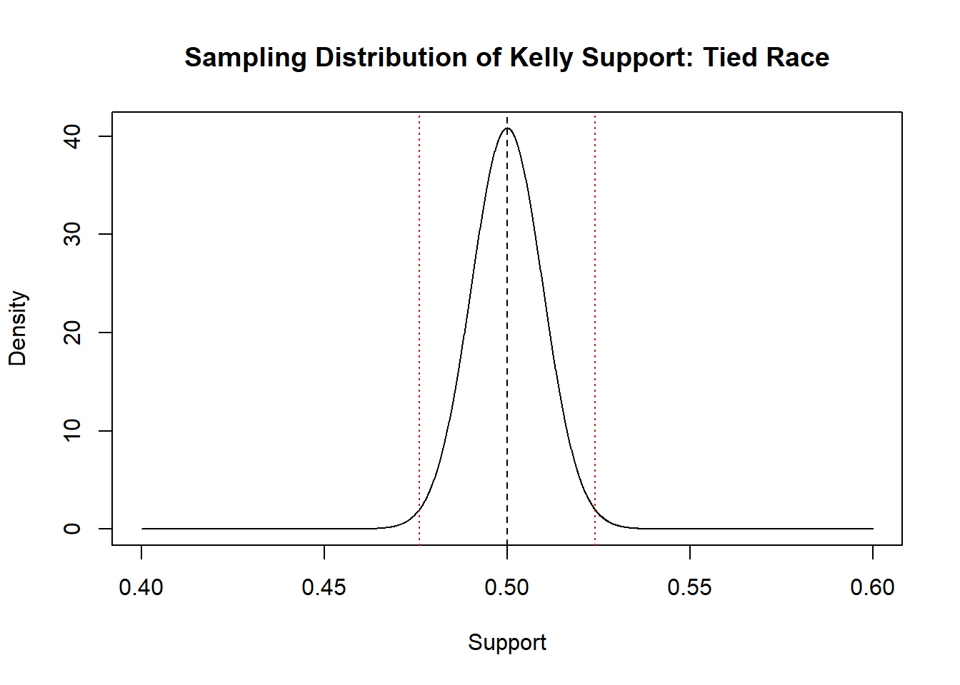
Just visually it seems like this is a tough call on whether we will reject the null hypothesis in this case. There is very few means that would be generated in the tails if the this was the sampling distribution that was producing means, but I can’t eyeball how many that might be.
- Compute the p-value (one sided or two sided).
Now we feel like we can use the normal distribution here because our n is sufficiently large:
But if we wanted to be really exact we could use the t-distribution. The t-distribution is like the standard normal in that it is a reference distribution. It tells us our answer in standard error units that we need to convert back in forth.
How many standard errors is our mean away from the null hypothesis:
t <- (.524-.5)/(s/sqrt(2613))Evaluate that number in the t-distribution with 2612 degrees of freedom:
pt(t, df=2612, lower.tail=F)*2
#> [1] 0.01411817
Same answer!
- Reject the null hypothesis if the p-value is less than or equal to \(\alpha\). Otherwise retain the null hypothesis.
We fail to reject the null hypothesis that the race is tied. A false negative!
To set up what we are going to talk about next time, how much do we get false negatives? We know that we will get false positives (reject the null when we shouldn’t) 5% of the time. That’s what we set up on purpose! But how does that translate into a false negative rate?
Given that the true percentage of Kelly’s vote is 52.4%, let’s simulate many polls of 2613 people, perform a hypothesis test on each, and determine what proportion of those tests are false negatives: where we fail to reject the null of 50%.
set.seed(19104)
false.negative <- rep(NA,10000)

n <- 2613
alpha <- .05

for(i in 1:10000){
samp <- rbinom(n,1, .524)
s <- sd(samp)
xbar <- mean(samp)
se <- s/sqrt(n)
t.val <- (xbar-.5)/se
p <- pt(t.val, df=n-1, lower.tail = F)*2
false.negative[i] <- p>=alpha
}
mean(false.negative)
#> [1] 0.3215
32% of the time we get a false negative! That’s a lot! Way higher than 5%. We call this value \(\beta\). We will start next time talking more about \(\beta\), but for right now: thinking about the sampling distribution under the null hypothesis, what might affect the size of \(\beta\)?
9.4 Review
Let’s do another example of a hypotheis test with some real data:
Here again is some real data for the final 2 weeks of our poll in Arizona:
library(rio)
sm.az <- import("https://github.com/marctrussler/IIS-Data/raw/main/AZFinalWeeks.csv")
head(sm.az)
#>   V1           id     weight week bi.week state county.fips
#> 1  1 118158025617 0.03165892   43      22    AZ        4013
#> 2  2 118157557679 0.89310665   43      22    AZ          NA
#> 3  3 114153878749 1.06902117   43      22    AZ          NA
#> 4  4 118159457343 0.07919169   43      22    AZ       25027
#> 5  5 118157881702 2.06085504   43      22    AZ          NA
#> 6  6 118158946302 3.62068552   43      22    AZ       36047
#>         senate.topline governor.topline      biden.approval
#> 1             Democrat         Democrat    Somewhat approve
#> 2                 <NA>             <NA>    Somewhat approve
#> 3                 <NA>             <NA> Somewhat disapprove
#> 4                 <NA>             <NA> Somewhat disapprove
#> 5 Other/Would not Vote       Republican    Somewhat approve
#> 6 Other/Would not Vote         Democrat                <NA>
#>   presvote2020         pid     ideology
#> 1          dem    Democrat     Moderate
#> 2          dem    Democrat Conservative
#> 3    dnv/other  Republican Conservative
#> 4    dnv/other Independent     Moderate
#> 5    dnv/other    Democrat      Liberal
#> 6    dnv/other  Republican     Moderate
#>   most.important.problem abortion.policy age     race
#> 1              Inflation            <NA>  37    black
#> 2       Crime and safety            <NA>  24    asian
#> 3              Inflation            <NA>  46 hispanic
#> 4              Inflation            <NA>  23    black
#> 5               Abortion            <NA>  28    black
#> 6                   <NA>            <NA>  77    white
#>   gender hispanic             education
#> 1   male    FALSE  Post graduate degree
#> 2   male     TRUE    Associate's degree
#> 3   male     TRUE      College graduate
#> 4 female    FALSE          Some college
#> 5 female    FALSE  Post graduate degree
#> 6   male    FALSE High school or G.E.D.
This time, let’s examine approval for Joe Biden in the Arizona electorate.
First, let’s create a variable that describes if someone approves of Joe Biden, or not.
table(sm.az$biden.approval)
#>
#>    Somewhat approve Somewhat disapprove    Strongly approve
#>                 665                 287                 623
#> Strongly disapprove
#>                1449
sm.az$approve.biden[sm.az$biden.approval %in% c("Strongly approve","Somewhat approve")] <- 1
sm.az$approve.biden[sm.az$biden.approval %in% c("Strongly disapprove","Somewhat disapprove")] <- 0
table(sm.az$biden.approval, sm.az$approve.biden)
#>
#>                          0    1
#>   Somewhat approve       0  665
#>   Somewhat disapprove  287    0
#>   Strongly approve       0  623
#>   Strongly disapprove 1449    0
#
mean(sm.az$approve.biden, na.rm=T)
#> [1] 0.4259259
sd(sm.az$approve.biden,na.rm=T)
#> [1] 0.4945644
sum(table(sm.az$approve.biden))
#> [1] 3024
3024 people answered this question. Of that sample, 42.6% of them stated that they approved of Biden (at least somewhat).
Again, 50% might be the relevant value for a null hypothesis here because we may want to know if Arizonans are ambivalent towards the President, or not. But to show that a null hypothesis can be anything, we could also test whether Biden’s approval rating is significantly different than Trump’s approval rating at the end of his term (38%).
Let’s go through the steps of testing this:
- Specify a null hypothesis and an alternative hypothesis.
\[ H_o: P(Approve.Biden)=.38\\ H_a: P(Approve.Biden)\neq.38 \]
- Choose a test statistic and the level of test (\(\alpha\)).
Our test statistic is the sample mean:
mean(sm.az$approve.biden,na.rm=T)
#> [1] 0.4259259
We will stick with \(\alpha=.05\).
- Derive the sampling distribution:
The sampling distribution is \(\frac{\bar{X_n}-E[X]}{s/\sqrt{n}} \sim t_{n-1}\)
The standard error is the standard deviation of the sampling distribution:
- Compute the p-value (one sided or two sided).
First, how many standard errors from the null is our test statistic:
t.score <- (mean(sm.az$approve.biden,na.rm=T)- .38)/seEvaluate the amount in the tail of the t distribution with 3023 degrees of freedom \(\pm\) that amount:
pt(t.score, df=3023, lower.tail=F)*2
#> [1] 3.484672e-07
Now this is a very, very low p-value. How should we report it? We could say that it is .0003%. That’s fine! Could we round down to 0? No! Never! A P value can never be zero! We are measuring the area under a curve and that curve assymptoptically approaches 0 but never hits it, so a p-value can never be precisely zero. My preference for very low p-values is to simply report them as “less than 1%”
- Reject the null hypothesis if the p-value is less than or equal to \(\alpha\). Otherwise retain the null hypothesis.
We reject the null hypothesis that Biden’s approval rating is equal to Trump’s last recorded approval rating. There is a less than a 1% chance of observing something as extreme as Biden’s 42% approval rating if the truth was that his approval rating was 38%.
Now I think it is important to know the steps of this process and what is happening under the hood because, honestly, it’s not that complicated.
We could write a function to take a sample, input a null hypothesis, calculate the standard error, look up the right probability bounds using pt and outputing a p-value….. But if that’s so easy to do someone’s probably already done it.
And yeah:
#Default is null=0
t.test(sm.az$approve.biden)
#>
#>  One Sample t-test
#>
#> data:  sm.az$approve.biden
#> t = 47.359, df = 3023, p-value < 2.2e-16
#> alternative hypothesis: true mean is not equal to 0
#> 95 percent confidence interval:
#>  0.4082918 0.4435601
#> sample estimates:
#> mean of x
#> 0.4259259
#Define our actual null hypothesis
t.test(sm.az$approve.biden, mu=.38)
#>
#>  One Sample t-test
#>
#> data:  sm.az$approve.biden
#> t = 5.1065, df = 3023, p-value = 3.485e-07
#> alternative hypothesis: true mean is not equal to 0.38
#> 95 percent confidence interval:
#>  0.4082918 0.4435601
#> sample estimates:
#> mean of x
#> 0.4259259
9.5 Power
Let’s think again about the possible outcomes of a hypothesis test.
- We could accept the null hypothesis when we shouldn’t (a false negative, \(\beta\)).
- We could accept the null hypothesis when we should (a true negative).
- We could reject the null when we shouldn’t (a false positive, \(\alpha\)).
- We could reject the null when we should (a true positive).
The thing we have control over here is \(\alpha\). It is what we explicitly set and therefore it is what we set it at. Keep in mind that 5% is…. pretty high! In my other job I work on the NBC news decision desk where our job is to explicitly reject the null hypothesis that the race is tied for the alternative hypothesis that a candidate has won. In 2022 we called around 600 races. If our standard was a 5% false positive rate we would get \(600*.05=30\) races wrong! We would absolutely lose our jobs. We say that we have an \(\alpha=.005\), but that would still be \(600*.005=3\) wrong calls. That would actually still be unacceptable.
\(\beta\), the probability of a false negative, is a bit more of a mystery. And we have to make some assumptions to get there.
What we want to answer is: What is the probability of concluding that Biden’s approval rating is not different from Trumps, if the truth is that it is different?
Put another way: if the truth is that Biden actually has a higher (or lower!) approval rating, what is the probability that we mistakenly conclude that the race is actually tied?
Right now we think we have a good idea on the shape of the sampling distribution (i.e. we know the standard error), and the move we have made for hypothesis testing is saying: what if they truth was 38%? What sort of means would be produced if that was the case?
This looks like this:
n <- 3024
hO <- .38
alpha <- .05
eval <- seq(.34,.44,.0001)
sd <- sqrt(hO*(1-hO))
seO <- sd/sqrt(3024)

plot(eval, dnorm(eval, mean=hO, sd=seO), type="l", col="darkblue", main="What is Beta?")
legend("topleft",c("Null Hyp. Sampling Distribution") , lty=c(1), col=c( "darkblue"))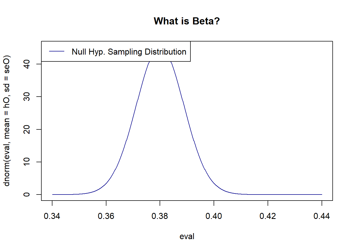
If the null hypothesis were true, this is the distribution that would be producing means. We can therefore determine the relatively likelihood of getting something like 38.5% (high) or 44% (low).
Now we want to add to this. Let’s posit a second possibility. What if the actual true population mean was 40%. If that was the case, what would that sampling distribution look like?
n <- 3024
hA <- .40
hO <- .38
alpha <- .05

sd <- sqrt(hA*(1-hA))
seA <- sd/sqrt(n)

plot(eval, dnorm(eval, mean=hA, sd=seA), type="l", col="firebrick", main="What is Beta?")
legend("topleft","True Sampling Distribution", lty=1, col="firebrick")
points(eval, dnorm(eval, mean=hO, sd=seO), type="l", col="darkblue")
legend("topleft",c("True Sampling Distribution","Null Hyp. Sampling Distribution") , lty=c(1,1), col=c("firebrick", "darkblue"))
Ok this is a little bit tricky, but let’s think about it this way. We are interested, as a research question, as to whether Biden’s approval rating is 38%, or not. This means that we would always have this distribution as our null hypothesis sampling distribution.
We are making a second preposition: what if the actual truth was 40%? If that was the case, then the red distribution would be the sampling distribution generating means.
For this null sampling distribution, in what range will we fail to reject the null hypothesis? The means that are in the 95% of the probability mass in the middle of the null distribution, between these two lines:
z.score <- qnorm(alpha/2)*-1
bounds <- c(hO+z.score*seO, hO-z.score*seO)


plot(eval, dnorm(eval, mean=hA, sd=seA), type="l", col="firebrick", main="What is Beta?")
legend("topleft","True Sampling Distribution", lty=1, col="firebrick")
points(eval, dnorm(eval, mean=hO, sd=seO), type="l", col="darkblue")
abline(v=bounds, lty=2, col="darkblue")
legend("topleft",c("True Sampling Distribution","Null Hyp. Sampling Distribution") , lty=c(1,1), col=c("firebrick", "darkblue"))
If we posit: the blue distribution is how we are testing our null hypothesis, but the red distribution is the one actually producing the means, we can now ask: what percentage of means generated by the red distribution will fall between the dotted blue lines? Put back into terms of the question: if the true level of Biden support is 40%, how often will we fail to reject the null hypothesis that the race is tied?
Alright so the red distribution is actually producing the means, while the blue distribution is what we are using for our hypothesis tests. It stands to reason that means produced in between the two blue lines by the red distribution will be the means that will mistakenly lead to failing to reject the null hypothesis.
So all we need to do is determine the probability mass of the red distribution that is between the two dotted blue lines:
Approximately 38% of the red distribution is in between the two blue lines. So 38% of the time the red distribution produces means that are in the region that will lead to the a failure to reject the null. In other words, the probability of a false negative is 38%!
Can we confirm this with a simulation:
library(dplyr)
false.negative <- rep(NA, 10000)

for(i in 1:10000){
  #Generate sample for truth of 40%
  samp <- rbinom(3204, 1, .4)
  #Perform hypothesis test using "within confidence interval" method
  false.negative[i] <- between(mean(samp), bounds[2], bounds[1])
}

mean(false.negative)
#> [1] 0.3687
Yeah about right!
Looking visually at the two distributions, it’s clear that there are several things that we can do to get less false positive:
The first (and stupidest) thing we can do is to have hA be further away from the null:
#Input
n <- 3024
hA <- .43
hO <- .38
alpha <- .05

#SE of alternative
sd <- sqrt(hA*(1-hA))
seA <- sd/sqrt(n)

#SE of Null
sd <- sqrt(hO*(1-hO))
seO <- sd/sqrt(n)

#Calculate rejection zone for alpha
z.score <- qnorm(alpha/2)*-1
bounds <- c(hO+z.score*seO, hO-z.score*seO)

eval <- seq(.34,.44,.0001)
plot(eval, dnorm(eval, mean=hA, sd=seA), type="l", col="firebrick", main="What is Beta?")
legend("topleft","True Sampling Distribution", lty=1, col="firebrick")
points(eval, dnorm(eval, mean=hO, sd=seO), type="l", col="darkblue")
abline(v=bounds, lty=2, col="darkblue")
legend("topleft",c("True Sampling Distribution","Null Hyp. Sampling Distribution") , lty=c(1,1), col=c("firebrick", "darkblue"))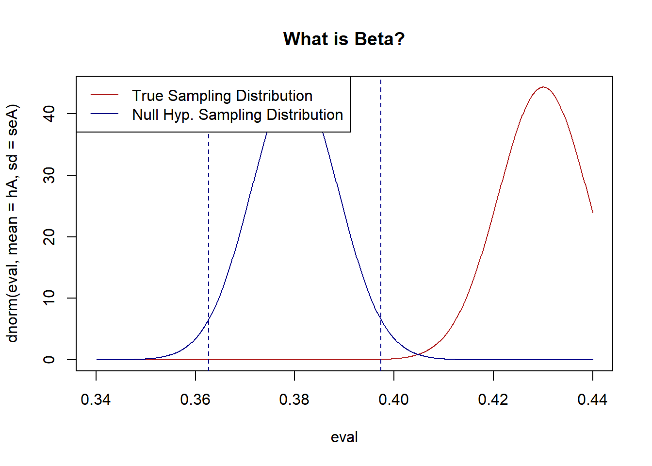
#Beta calculation:
pnorm(bounds[1], mean=hA, sd=seA) - pnorm(bounds[2], mean=hA, sd=seA)
#> [1] 0.0001405171
These two distributions are the same shape as above, but now the “truth” is that Biden approval is 43%. Because this is simply further away from the null then we are much less likely to get a false negative. Taken to the extreme: if everyone approved of Biden there obviously would be no chance of getting a false negative as we would never get anywhere close to thinking that 38% of people supported him.
But given that the truth is fixed, we can also think about changing other parameters to lower our false positive rate.
First, if we raise the false negative rate, \(\alpha\) we will have a lower false positive rate. That looks like this:
#Input
n <- 3024
hA <- .4
hO <- .38
alpha <- .1

#SE of alternative
sd <- sqrt(hA*(1-hA))
seA <- sd/sqrt(n)

#SE of Null
sd <- sqrt(hO*(1-hO))
seO <- sd/sqrt(n)

#Calculate rejection zone for alpha
z.score <- qnorm(alpha/2)*-1
bounds <- c(hO+z.score*seO, hO-z.score*seO)

eval <- seq(.34,.44,.0001)
plot(eval, dnorm(eval, mean=hA, sd=seA), type="l", col="firebrick", main="What is Beta?")
legend("topleft","True Sampling Distribution", lty=1, col="firebrick")
points(eval, dnorm(eval, mean=hO, sd=seO), type="l", col="darkblue")
abline(v=bounds, lty=2, col="darkblue")
legend("topleft",c("True Sampling Distribution","Null Hyp. Sampling Distribution") , lty=c(1,1), col=c("firebrick", "darkblue"))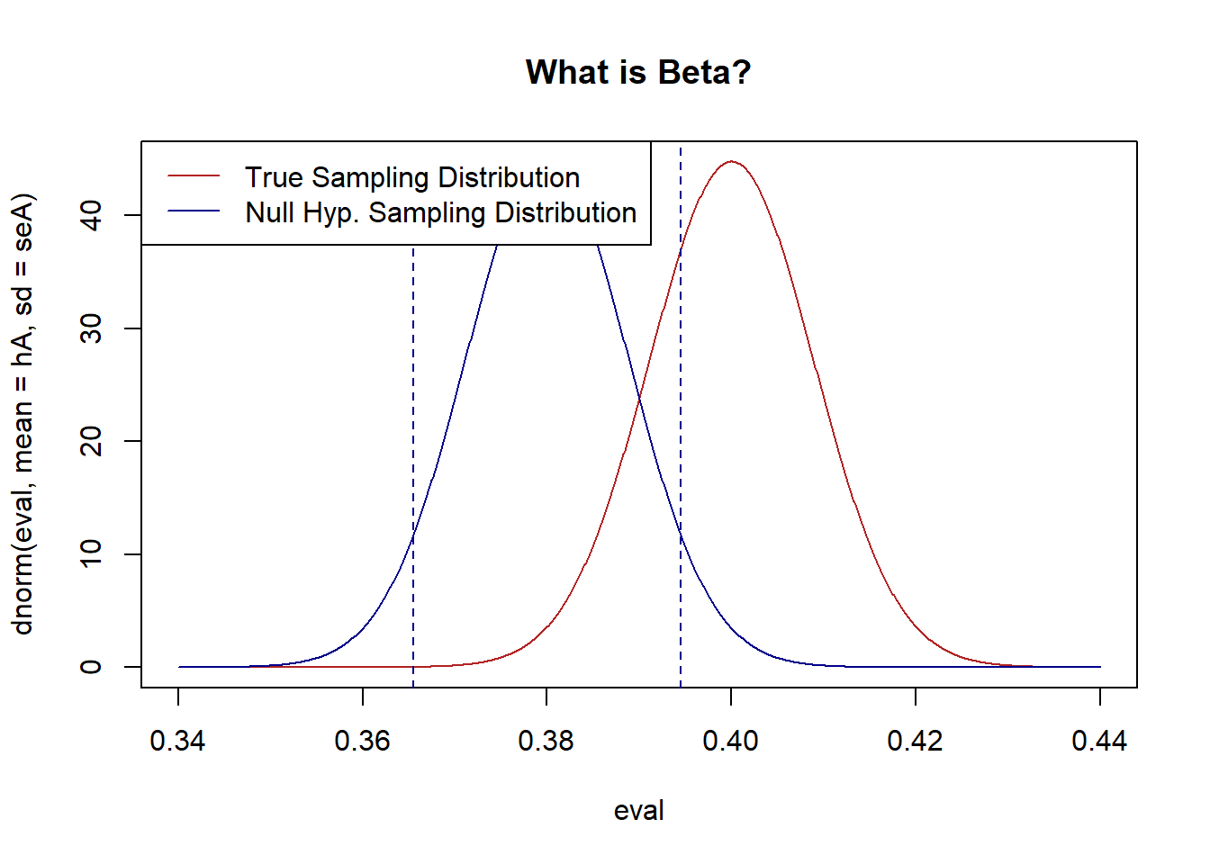
#Beta calculation:
pnorm(bounds[1], mean=hA, sd=seA) - pnorm(bounds[2], mean=hA, sd=seA)
#> [1] 0.2691288
The area between the two lines is now somewhat smaller, and as such the probability that a mean from the red area is produced in that zone is smaller. We see that this drops the false negative rate to 27%.
The other thing that we can do is to reduce the width of the sampling distributions. Then, for a given level of alpha and a given difference between the truth and the null hypothesis there will be less overlap between the two distributions.
The easiest way to do this is to increase the sample size. Let’s increase the sample size to 5000 people:
#Input
n <- 5000
hA <- .4
hO <- .38
alpha <- .05

#SE of alternative
sd <- sqrt(hA*(1-hA))
seA <- sd/sqrt(n)

#SE of Null
sd <- sqrt(hO*(1-hO))
seO <- sd/sqrt(n)

#Calculate rejection zone for alpha
z.score <- qnorm(alpha/2)*-1
bounds <- c(hO+z.score*seO, hO-z.score*seO)

eval <- seq(.34,.44,.0001)
plot(eval, dnorm(eval, mean=hA, sd=seA), type="l", col="firebrick", main="What is Beta?")
legend("topleft","True Sampling Distribution", lty=1, col="firebrick")
points(eval, dnorm(eval, mean=hO, sd=seO), type="l", col="darkblue")
abline(v=bounds, lty=2, col="darkblue")
legend("topleft",c("True Sampling Distribution","Null Hyp. Sampling Distribution") , lty=c(1,1), col=c("firebrick", "darkblue"))
#Beta calculation:
pnorm(bounds[1], mean=hA, sd=seA) - pnorm(bounds[2], mean=hA, sd=seA)
#> [1] 0.1723704
Or to 10000 people:
#Input
n <- 10000
hA <- .4
hO <- .38
alpha <- .05

#SE of alternative
sd <- sqrt(hA*(1-hA))
seA <- sd/sqrt(n)

#SE of Null
sd <- sqrt(hO*(1-hO))
seO <- sd/sqrt(n)

#Calculate rejection zone for alpha
z.score <- qnorm(alpha/2)*-1
bounds <- c(hO+z.score*seO, hO-z.score*seO)

eval <- seq(.34,.44,.0001)
plot(eval, dnorm(eval, mean=hA, sd=seA), type="l", col="firebrick", main="What is Beta?")
legend("topleft","True Sampling Distribution", lty=1, col="firebrick")
points(eval, dnorm(eval, mean=hO, sd=seO), type="l", col="darkblue")
abline(v=bounds, lty=2, col="darkblue")
legend("topleft",c("True Sampling Distribution","Null Hyp. Sampling Distribution") , lty=c(1,1), col=c("firebrick", "darkblue"))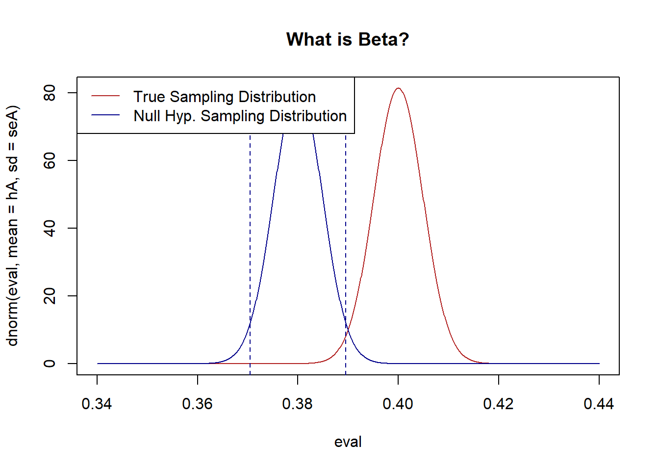
#Beta calculation:
pnorm(bounds[1], mean=hA, sd=seA) - pnorm(bounds[2], mean=hA, sd=seA)
#> [1] 0.01615443
The false negativity rate drops off substantially.
Given that the width of the sampling distribution is given by \(s/\sqrt{n}\) clearly we can either increase \(n\) or decrease \(s\) to make the sampling distribution smaller. In the case where we are sampling a bernoulli it’s very difficult to make \(s\) smaller, but it might be in other cases. For example a common survey question we ask are “Feeling Thermometers” where we ask people to rate how warmly they feel about a politician/group where 0 is cold and 100 is warm. As it turns out people are really bad at answering these questions and they have a lot of random variation. All things being equal, that high variance question is going to lead to a higher \(\beta\).
When we are performing research we often don’t think in terms of \(\beta\), but instead consider \(1-\beta\), which we call “statistical power”. If \(\beta\) is the probability of failing to reject the null hypothesis when we should, then power is the probability of rejecting the null hypothesis when we should. Put in other words, it’s our ability to say that something is there when something is in fact there.
Here’s an absurd example: Biden’s highest approval rating was 55%. Let’s say a survey firm completes a random survey of 15 people, generates an approval rating for Biden, but claims that they can’t conclude whether or not Biden is more popular than Trump was when he left office with a approval of 38%.
Let’s use the technique above to map out the true and null hypotheses for this firms test:
#Input
n <- 15
hA <- .55
hO <- .38
alpha <- .05

#SE of alternative
sd <- sqrt(hA*(1-hA))
seA <- sd/sqrt(n)

#SE of Null
sd <- sqrt(hO*(1-hO))
seO <- sd/sqrt(n)

#Calculate rejection zone for alpha
z.score <- qnorm(alpha/2)*-1
bounds <- c(hO+z.score*seO, hO-z.score*seO)

eval <- seq(.1,.7,.0001)
plot(eval, dnorm(eval, mean=hA, sd=seA), type="l", col="firebrick", main="What is Beta?")
legend("topleft","True Sampling Distribution", lty=1, col="firebrick")
points(eval, dnorm(eval, mean=hO, sd=seO), type="l", col="darkblue")
abline(v=bounds, lty=2, col="darkblue")
legend("topleft",c("True Sampling Distribution","Null Hyp. Sampling Distribution") , lty=c(1,1), col=c("firebrick", "darkblue"))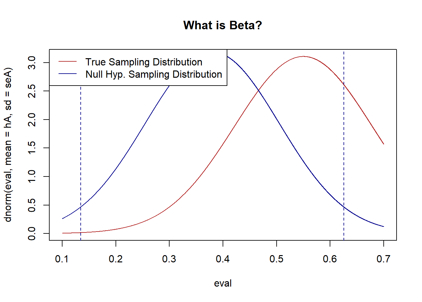
#Beta calculation:
pnorm(bounds[1], mean=hA, sd=seA) - pnorm(bounds[2], mean=hA, sd=seA)
#> [1] 0.7214013
With 15 people we have an enormously wide zone where we will fail to reject the null hypothesis. A wide band that is necessary to ensure our 5% false positive rate. We need extraordinary evidence to claim that a sample mean is different from 38% when we only have 15 people. Accordingly, we get a huge number of false negatives! Indeed, it’s more likely than not we will get a false negative.
Next week when we get to difference in means tests we will similarly be able to calculate the minimum detectable effect size given the \(n\) of an experiment, for example. An extraordinarily common critique of experiments is that authors failed to run a power analysis and, given the effect size that is plausible and their \(n\), they simply lacked the statistical power to find anything!
Similarly common in experiments is to what we saw above: authors may say: we ran an experiment and found nothing, so we conclude that nothing is there. But a lot of times power analysis will reveal that a 20 or 30% false negativity rate is expected. You can’t claim that nothing is happening when you get a result of “nothing” 30% of the time!
Can you have too much power? Not really, but the results of too much power can be somewhat misleading. Let’s say the true proportion of people who support Joe Biden is 38.5%, and a firm runs a poll with 1 million people in it. They get a result and conclude that Joe Bidens support is significantly different than Donald Trump’s low point of 38%. What would that look like:
#Input
n <- 1000000
hA <- .385
hO <- .38
alpha <- .05

#SE of alternative
sd <- sqrt(hA*(1-hA))
seA <- sd/sqrt(n)

#SE of Null
sd <- sqrt(hO*(1-hO))
seO <- sd/sqrt(n)

#Calculate rejection zone for alpha
z.score <- qnorm(alpha/2)*-1
bounds <- c(hO+z.score*seO, hO-z.score*seO)

eval <- seq(.34,.44,.0001)
plot(eval, dnorm(eval, mean=hA, sd=seA), type="l", col="firebrick", main="What is Beta?")
legend("topleft","True Sampling Distribution", lty=1, col="firebrick")
points(eval, dnorm(eval, mean=hO, sd=seO), type="l", col="darkblue")
abline(v=bounds, lty=2, col="darkblue")
legend("topleft",c("True Sampling Distribution","Null Hyp. Sampling Distribution") , lty=c(1,1), col=c("firebrick", "darkblue"))
#Beta calculation:
pnorm(bounds[1], mean=hA, sd=seA) - pnorm(bounds[2], mean=hA, sd=seA)
#> [1] 4.383925e-17
It’s extraordinarily unlikely to get a false negative when you have an \(n\) that big, and as such very small differences from the null can be said to be “statistically significant”. But here is where we get into the art rather than the science of statistics, just because something is statistically significant doesn’t mean that it is substantively significant. I don’t think that anyone would claim that an approval rating of 38.5% is substantively different than an approval rating of 38%. You can get a very large sample and conclude that something is statistically significant, but that says nothing about the relative magnitude or importance of that effect.
My other favorite example of this is meat cancer. And by favorite I mean a god-damn disaster of science communication. Whole industries were launched, careers made, and documentaries written by the fact that the WHO labeled red meat a “Group 1” carcinogen, the same group that “arsenic, asbestos, and tobacco belong to”.
What was happening here? Is red meat as damaging to you as smoking? No! Not even close.
What happened was that there was a large accumulation of studies that, in total, showed that red meat had a small effect on the rates of colon cancer. The WHO’s “Group 1” is not a measure of how severe a carcinogen is, but is a measure of statistical significance. Enough studies had been done that there was sufficient evidence to overturn the null hypothesis that meat did not effect the rate of cancer.
Because people generally don’t think like this, people assumed what the WHO meant was that bacon was just as harmful as smoking.
Side bar 1: The meat cancer scare was helped along by some truly weird choices by the epidemiologists about how to communicate the risk. All the headlines stated that “Eating 50g of processed meat a day increases the risk of colon cancer by 18%” A reasonable person would think that, if the baseline rate of colon cancer is 3%, then eating 50g of processed meat a day would lead to a rate of colon cancer of 3+18=21%. But that’s not at all what they were saying, they were saying that if the baseline rate of colon cancer was 3%, then eating 50g of processed meat a day would lead to a race of colon cancer of 3*1.18=3.54%. The 18% was a “relative risk” calculation, not a change in percentage points. That’s a lot less dramatic!
Let’s compare that to another “Group 1” carcinogen. The probability of lung cancer for never smokers is approximately .015%, that is, 1 in 1000. The probability of lung cancer for smokers is approximately 25%, that is, 1 in 4. As such, compared to the “18%” relative risk of colon cancer from meat, there is a 1666% relative risk increase of lung cancer from smoking.
So if anyone tells you that eating meat is as dangerous as smoking, tell them Dr. Trussler said that they are a clown.
That being said we should probably all cut back on our red and processed meat consumption :).
Side bar 2: If everyone misinterprets what you said as a scientist, it’s not their fault, it’s your fault.