5 Continuous Random Variables
Thus far the two types of variables that we looked at were discrete random variables. This covers a good number of outcomes, but many other things we are interested in are continuous. This gives us the second class of RVs to think about.
By definition, a continuous random variable can take on an infinite number of values between two intervals.
Something being continuous gives some additional problems… problems that unfortunately will require the help of calculus to solve (though we are going to let R do most of the math for us!).
5.1 Uniform Random Variables
The simplest continuous random variable is the uniform random variable. Simply: the uniform random variable says that all points within a given interval are equally likely to occur.
A good example is births throughout the year. Consider being born at some point between day 1 and day 365 in the year, if we were to make a graph of the odds of being born at any point throughout the year it would look like:
plot(c(-10,375), c(0,1.5/365), type="n",
     xlab="Birth Time", ylab="Density")
segments(-10,0,1,0)
segments(1,1/365,365,1/365)
segments(365,0,380,0)
points(c(0,365), c(0,0))
points(c(1,365), c(1/365, 1/365), pch=16)
To be clear here, we are not “rounding” each person to their birth date. That would be a discrete uniform RV because the days o the year are countable and would have a PMF of something like:
\[ f(K) = p(K=k) = \begin{cases} \frac{1}{365} \text{ if } 1\\ \frac{1}{365} \text{ if } 2\\ \frac{1}{365} \text{ if } 3\\ \dots \\ \frac{1}{365} \text{ if } 365\\ \end{cases} \] [Draw the PMF]
[Draw the CDF]
Instead here we are thinking of time in a continuous fasion, and considering the actual moment of birth as the realization of this random variable.
For this continuous variable (and for all continuous variables) there are an infinite number of possible moments of birth. You can be born at dat 3.1, or day 5.12, or day 5.182191710371918…..
This, however, immediately presents a problem for how we have defined Random Variables thus far. We have defined these such that the probability of all possible events sums to 1.
But if there are an infinite number of possible birth moments, then if the probability of any specific time is greater than 0 that the sum of all the events will also be infinity.
For that reason, in a continuous probability distribution the probability of any specific number is equal to 0. “Measurement Theory” is the branch of mathematics that solves these sorts of problems (with calculus). For right now it is enough to say that every point in the uniform interval has probability 0 but “positive measure”.
In that way we can draw the distribution we drew above.
For a discrete variable, this distribution (which tells us the probability of any particular point occurring) was a Probability Mass Function or PMF. For continuous random variables this same graph is a Probability Density Function, or PDF.
For a uniform RV the pdf is defined as
\[ f(X) = \begin{cases} \frac{1}{b-a} \text{ if } a\leq x \leq b\\ 0 \text{ otherwise} \end{cases} \]
How can we get the CDF of this PDF?
We can’t sum up all of the individual times of the year because there are an infinite number. So our previous equation of \(F[x] = \sum f(X \leq x)\) won’t work.
Instead we turn to calculus. For a continuous RX the CDF is equal to \(F(x) = \int_{-\infty}^{x} f(x) \partial x\). We integrate the PDF (add up the area under the curve) from negative infinity to the value that we care about.
For the uniform random variable we have been discussing that would look like:
The two functions (PDF and CDF) are still directly completments of one another, such that if you know one you automatically know the other.
We just saw that the CDF is the integration of the PDF. So clearly given a PDF we can create the CDF.
But the opposite is true to. Given a CDF, the value of the PDF at any corresponding point is the first derivative of the CDF at that point.
If you are unfamilar with calculus (or rusty), the first derivative just means the slope at that point.
Looking at these charts for the uniform random variable, the slope of the CDF is 0 everywhere below 0 and above 365. In between the slope is a constant \(\frac{1}{b-a}\).
In R we can use the dunif() and punif() commands to consider a uniform RV.
Looking at the help file, we use min and max to set the bounds of the Uniform RV, and R knows that those things are equal in between those points.
We can get R to draw the PDF and CDF of the uniform distribution by providing those functions the relevant values.
#?dunif

#Draw the PDF of the birthday Uniform
points <- seq(-50,410,.01)

plot(points, dunif(points, min=1, max=365), type="l",
     main="PDF of Uniform Variable",
     xlab="Value",
     ylab="density")
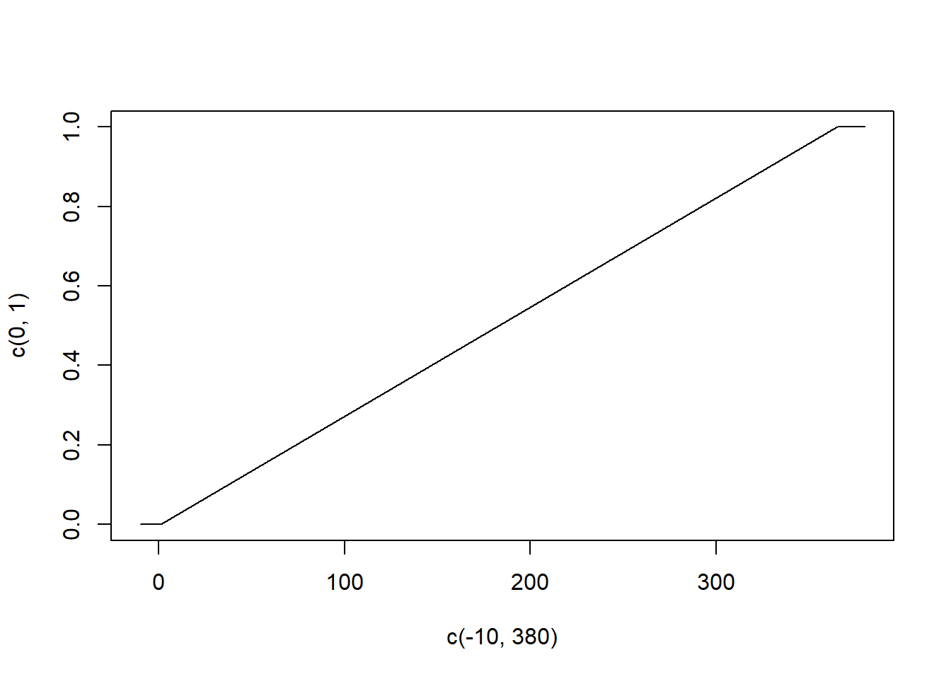
plot(points, punif(points, min=1, max=365), type="l",
     main="PDF of Uniform Variable",
     xlab="Value",
     ylab="density")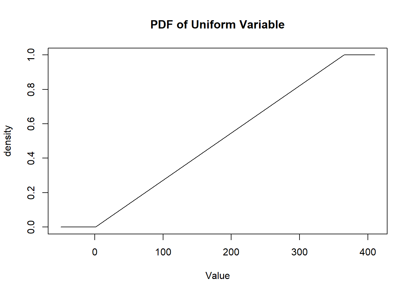
We can also use the runif() function to make random draws from this distribution.
Again, this will draw from the continuous uniform distribution, so we will not get integer values when we use it. So for example drawing 10 “birth-times”:
runif(10,1,365)
#>  [1] 356.70630  91.55504  73.90451  71.04125 243.36051
#>  [6] 169.62313 199.72162 151.06060 110.49047 204.01103
But drawing birthdays from a discrete uniform variable is easy! And indeed you’ve been doing it when you worked on the birthdya problem or did anything with dice rolls.
To get the expected value of a continuous random variable we do the same procedure of adding up all of the values multiplied by the probability the RV takes on that value. But, because we can’t to that literally (because the probability of any given point is 0 and there are infinite number of points) we use calculus.
So \(E[X] = \int_a^b x*f(x) \partial x = \text{Math!} = \frac{a+b}{2}\).
Similarly for variance you would go through a similar procedure and get: \(V[X] = E[X^2] - E[X]^2 = \text{Math!} = \frac{1}{12}(b-a)^2\)
5.2 The Normal Random Variable
The second continuous RX we are going to look at is the Normal Distribution. Also known as the “Gaussian” Distribution.
It’s the most important distribution! It’s famous!
More on its importance in a moment, but first some definitions: the normal distribution is the bell shaped distribution you know well (draw). It takes on any value from negative infinity to positive infinity.
It is always symmetrical around its midpoint, which is defined as the greek letter \(\mu\). This symmetrical feature will be very important in the coming weeks. We can think of it as 50% of the probability mass is to the left of the midpoint and 50% of the probability mass is to the right of the midpoint. This means that \(\mu\) is both the mean and median of the distribution!
The PMF of the normal distribution is defined as:
\[ f(x) = \frac{1}{\sqrt{(2\pi \sigma)}} e^{- \frac{1}{2\sigma^2}(x-\mu)} \]
So that’s terrible! In no way do you have to know this formula or ever think of it again. What is critical though is that the normal distribution can be drawn for any value of x based on two values: \(\mu\) and \(\sigma\).
\(\mu\) we have seen is simply the expected value of a normal random variable, while \(\sigma^2\) is simply the variance of the normal distribution.
Put opposite: if you give me the \(\mu\) and \(\sigma\) of a normal distribution, I can (well, R can…) draw it exactly via that formula below.
And we can see in R that if we provide a mu and a sigma it will shoot back the density for any values that we enter.
#?dnorm
values <- seq(-100,100,.001)
plot(values, dnorm(values, mean=0, sd=10), main="PDF of Normal Distribution mean 0 , sd=10",
type="l", xlim=c(-100,100))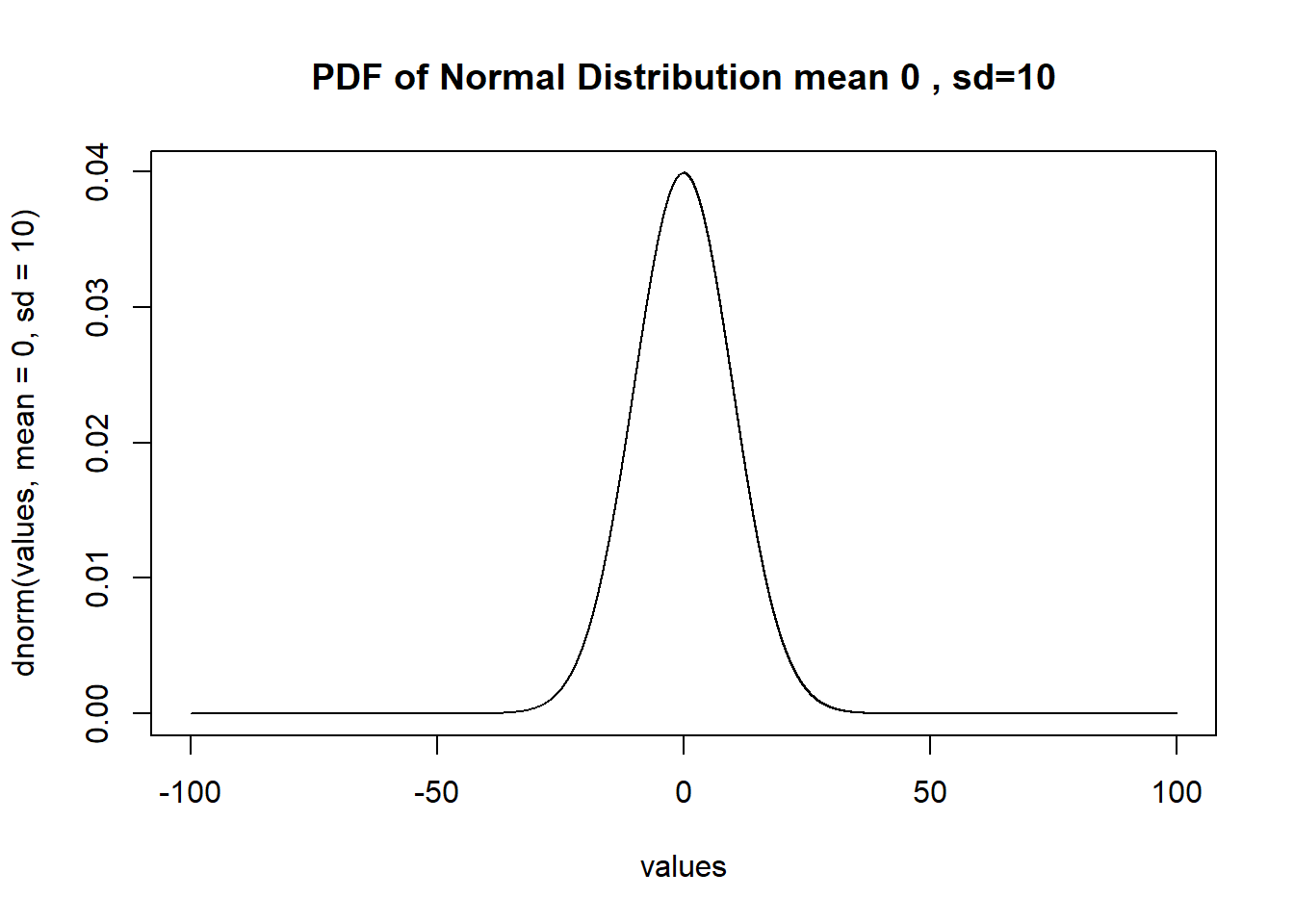 The CDF of a normal distribution is similarly defined as the integration from negative infinity to any given point of X. Like the CDF of the uniform distribution it starts at 0 and ends up at 1. However, because the density of standard normal is not equal across a given interval, the slope of the CDF will also vary. For example, here is the CDF for the normal distribution we just drew.
#?dnorm

values <- seq(-100,100,.001)
plot(values, pnorm(values, mean=0, sd=10), main="CDF of Normal Distribution mean 0 , sd=10",
     type="l", xlim=c(-100,100))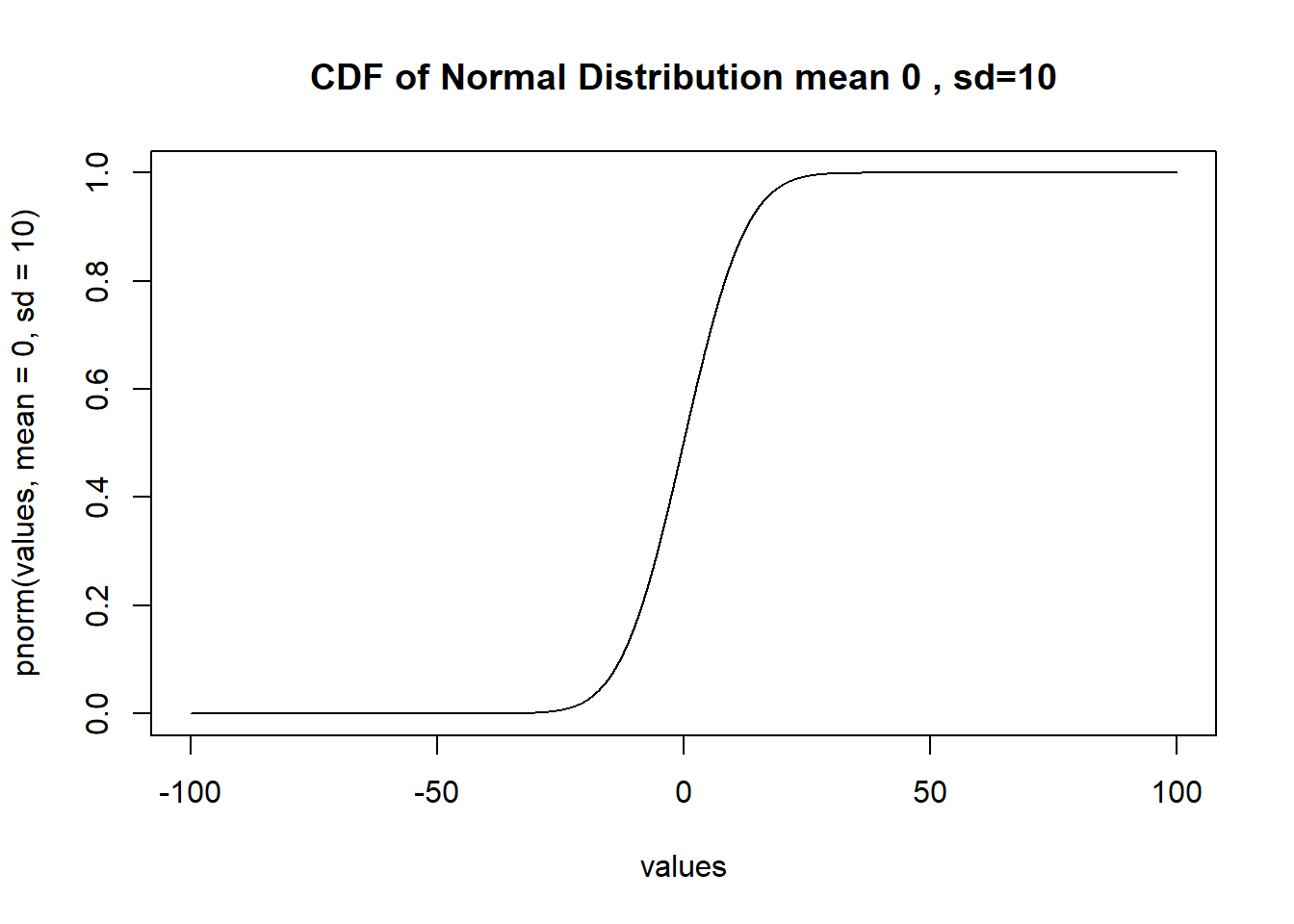
We won’t show it here, but the first derivative of any point of that CDF curve is the density at the same point in the PDF curve.
The final consideration I want to talk about for the normal distribution today is that the variance of the normal distribution is not related to the expected value. We saw for a binomial, for example, that the variance decreases as the probability of success goes up or down. The same is not true for a normal distribution. The \(\sigma\) of the standard normal completely determines the “shape”, while the \(\mu\) determines the location:
plot(values, dnorm(values, mean=0, sd=10), main="PDF of Normal Distribution mean(-50,0,50) , sd=10",type="l", xlim=c(-100,100))
points(values, dnorm(values, mean=-50, sd=10), type="l")
points(values, dnorm(values, mean=50, sd=10), type="l")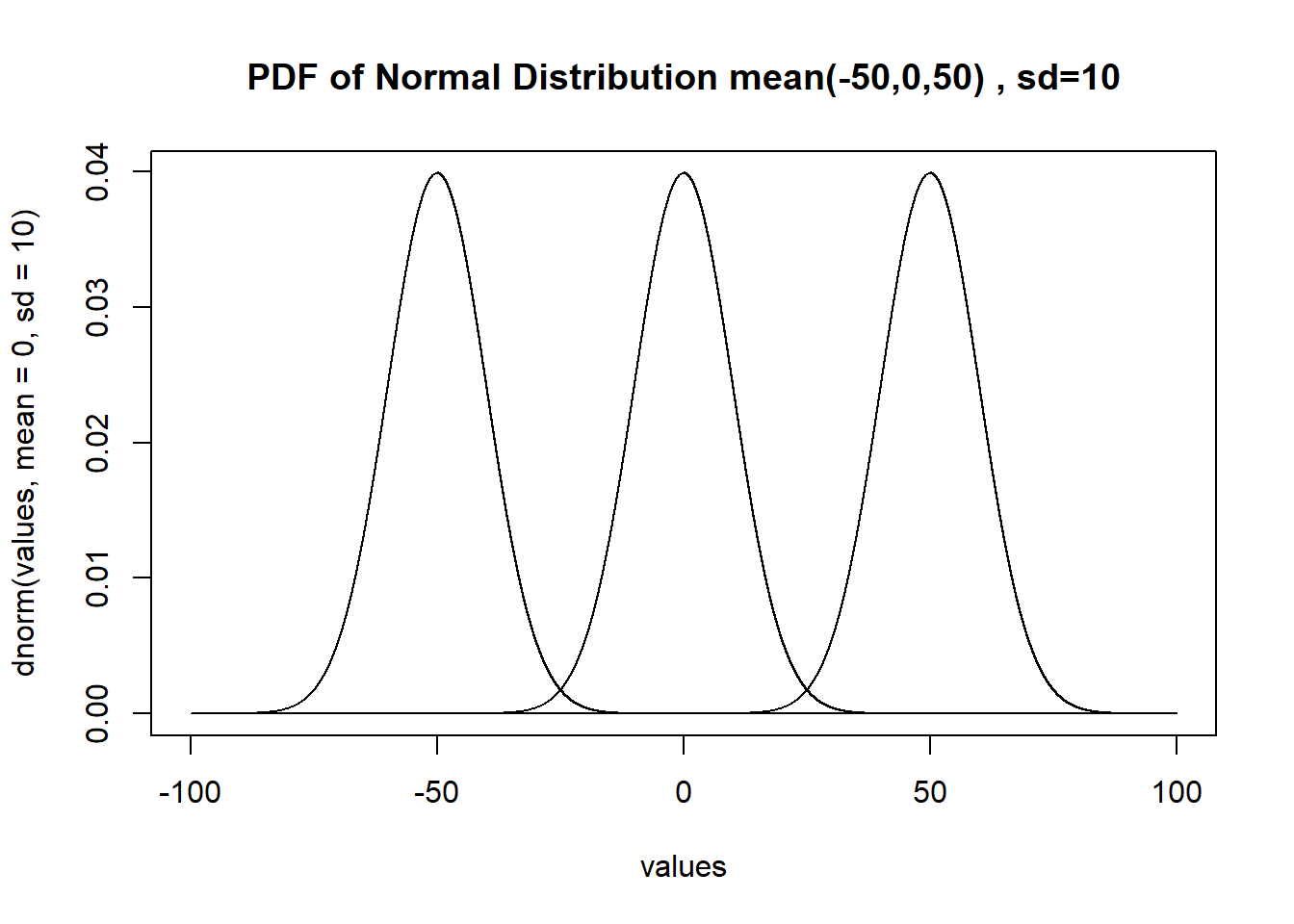
plot(values, pnorm(values, mean=0, sd=10), main="CDF of Normal Distribution mean(-50,0,50) , sd=10",type="l", xlim=c(-100,100))
points(values, pnorm(values, mean=-50, sd=10), type="l")
points(values, pnorm(values, mean=50, sd=10), type="l")
We are going to do lots more to consider the Nature of the normal distribution on Wednesday, but let’s finish up by thinking about : Why is it so important? Two reasons
- Many naturally occurring things are normally distributed. For example height is normally distributed. Here is the normal distribution for womens height in the US:
- Even more important: the “sampling distribution of nearly all of the statistics that we care about are normally distributed.
This is not something you understand right now, but it’s helpful to have this context before we spend a bit of time working with normal distributions.
Let’s say we are conducting a survey of 1000 and want to determine the proportion of people who approve of Joe Biden. Let’s pretend that we are God here and know that the true proportion of people who approve of Joe Biden is 44%. Clearly, each survey respondent’s answer is a bernoulli RV with probability of success or .44, so we can use the binomial distribution to pull 1000 people.
Here is one survey of 1000 people:
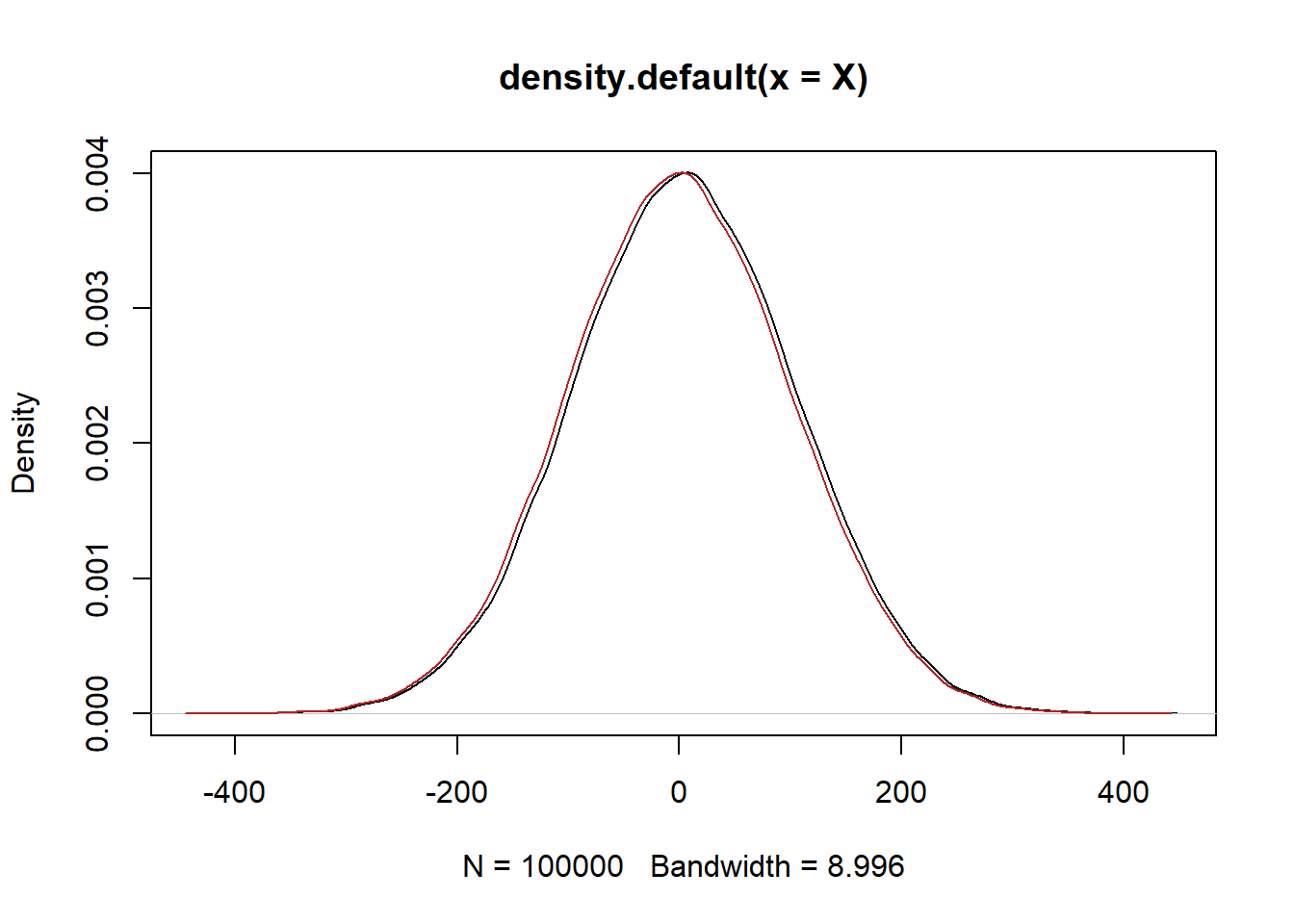
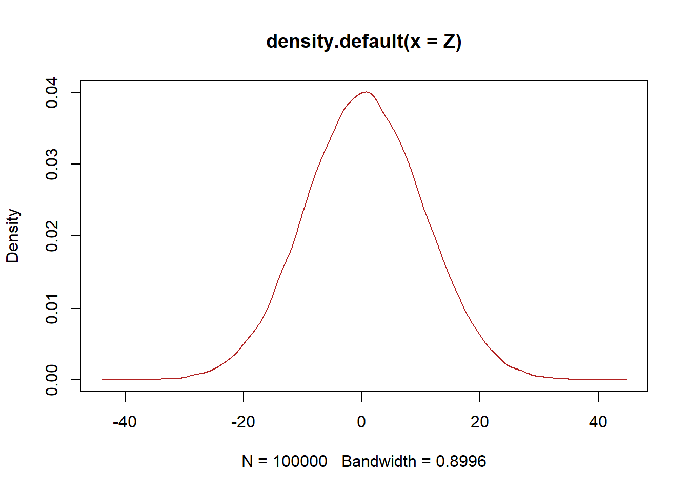
In the first sample we got 439 “successes”, so 43.9% of people support Joe Biden in this sample. We know that this number will be a little bit different every time, but it’s not super clear how different it will be each time. Let’s take 5000 samples of 1000 people and look at the distribution of all of sample means that we generate:

The distribution of all of the sample means drawn from a binomial variable is normally distributed (and we will see, with a known shape).
5.3 The Standard Normal
We left off last class discussing how the variance of a normal variable does not change if you add a constant to that variable.
Another way that we can express this is that if we simply add a constant to a RV it does not change the variance, it just shifts up and down the number line. Formally: if \(Z=X+c\) then \(Z \sim N(\mu+c, \sigma^2)\).
So if we have a random variable X that is normally distributed with mean 5 and standard deviation 100 and subtract 5 from every value:
It’s the same shape just shifted over by 5 units.
A second key mathematical feature of the normal distribution is that if we multiply or divide a normal variable by a constant, than what remains is also a normal distribution, where both \(\mu\) and \(\sigma^2\) are divided by that constant.
Formally: if \(Z=cX\) then \(Z \sim N(c\mu, c\sigma^2)\).
So if we take X and divide it by 10, the result is still a normal distribution, just caled down.

Those seem like two pretty useless facts…. however they let us make the following transformation to any random variable:
\[ Z = \frac{X-\mu}{\sigma} \]
If we take any normal distribution and (1) subtract off \(\mu\) from each value and divide the standard deviation by \(\sigma\) , we are definitionally left with another normal distribution. In particular, we are left with a normal distribution with mean=0 and sd=1. (It also has variance 1 because \(1^2=1\))
Following the rules we have set out:
If \(X \sim N(\mu=5,\sigma=100)\). To subtract a constant we subtract from \(\mu\) (it doesn’t affect the variance), so that would be \(\mu=0\). And then if we divide by 10 \(\mu=0\) (0 divided by anything is 0), and we are dividing \(\sigma\) by itself so that equals 1.
This transformation – subtract off the mean and divide by the standard deviation – transforms any normal random variable into the “standard” normal variable. The standard normal variable is a normal random variable with mean 0 and variance (and standard deviation) of 1.
Indeed, if you look at the help file for dnorm() you will see that the default values for mean and sd are 0 and 1. That is, the norm functions default to giving you information about the standard normal.
#?dnormThere are some key features of the standard normal distribution that we can think about through the pnorm() command.
The first question we want to answer is: What is the value of the CDF when Z=1.
[Draw Standard Normal PDF and CDF]
To determine this we can use the pnorm function, which is our method of interrogating the CDF:
The cumulative probability to the left of 1 in the standard normal is around 84.1%.
Just to pause for a second, what does this answer do, and why is that wrong:
dnorm(1)
#> [1] 0.2419707
This gives the approximate probability of drawing 1 from a standard normal distribution (i.e. the probability of 1 in the PDF).
OK so if .841 probability is to the left of 1 in the standard normal distribution, how much probability is to the right of 1?
Well we know that the total probability adds up to 1, so by definition the probability to the right of 1 must be \(1 -.841=.159\).
OK so here is a key question that we already have all the tools to understand: how much probability mass is to the left of negative 1?
Remember: the normal distribution is symmetrical! That’s its key feature. Because of that, there is by definition also .159 to the left of negative 1.
OK: last stretch here. How much probability mass is in between -1 and 1 in the standard normal?
Well, again, the total probability mass adds up to 1, so to get this answer we can do \(1 - 2*.159 = .683\).
In between -1 and 1 in the standard normal there is 68.3% of the probability mass.
How could we get the answer to this question in one line of code in R?
Using the principle that the normal distribution is symmetrical, we can do:
1-2*pnorm(-1)
#> [1] 0.6826895
What do we get if we do:
1-2*pnorm(1)
#> [1] -0.6826895
Clearly wrong! Use your head with probability. It MUST range between 0 and 1 so if you got this answer you know it would be wrong.
Now that we have a method, how much probability mass is \(\pm 2\) and \(\pm 3\) around \(\mu\) in the standard normal. Applying the same method:
95% of the probability mass is within \(\pm 2\) of \(\mu\) and 99.9% of the probability mass is within \(\pm 3\) of \(\mu\) in the standard normal.
Why does this matter!? Why are we doing this!?
What is \(\pm\) 1 for the standard normal distribution? It is it’s standard deviation (and variance). This means that 68.3% of the probability mass is within \(\pm 1\) standard deviations from \(\mu\) in the standard normal.
But think again: how did we derive the standard normal in the first place? We said that any normal distribution can be converted into the standard normal distribution by subtracting \(\mu\) from every value and dividing by \(\sigma\). This means that for the standard normal, 1 “unit” is one standard deviation. Let’s go through this slowly: If we have a normal distribution \(X \sim N(\mu=5, \sigma=10)\). If we think about the interval from 0 to 1 in the standard normal, what is the equivalent interval in X? In the standard normal going from 0-1 is going from \(\mu\) to \(\mu + \sigma\). Because all normal distributions are the same “shape” (just transformed to different widths), this same interval is \([\mu,\mu+\sigma] = [5,15]\). This means for our normal distribution X, there is 68.3% probability ,mass in the interval from \([-10,15]\), i.e. \(\pm \sigma\) around \(\mu\).
It should be clear now that because any normal distribution can be turned into the standard normal, and because there is 68.3% probability mass between -1 and 1 in the standard normal, there is 68.3% probability \(\pm \sigma\) for any normal distribution. (And similarly 95% \(\pm 2*\sigma\) and 99.9% \(pm 3*\sigma\)). This is called the empirical rule.
So If I told you that women’s height in the US was \(\sim N(\mu=64, \sigma^2=9)\), what interval contains approximately 95% of all women?
That is the interval that is \(\pm 2*\sigma\), which in this case equals \([\mu - 2*\sqrt{9}, \mu + 2*\sqrt{9}] = [58,70]\).
This also gives us a common language to talk about all normal distributions. When we talk about how many \(\sigma\)’s something is away from \(\mu\) we talk about it as a Z-score.
For example what is the Z-score for the distribution of women’s height of 73? To answer this we have to determine how many \(\sigma\)’s this is from \(\mu\): \(Z=\frac{73 - \mu}{\sigma} = \frac{73-64}{3} = 3\).
What is the probability that a women is under 73 inches tall?
Now to get that we can do:
pnorm(3)
#> [1] 0.9986501
To be clear, we should get the exact same answer if we do:
pnorm(73, mean=64, sd=3)
#> [1] 0.9986501
And we do.
OK so if I asked you to determine the probability above, why would you ever go through the hassle of converting it to a Z-score and calculating in that way when you can just put in the normal distribution shape that we care about and determine the right answer? Well…. you wouldn’t. So why do we have the standard normal and Z-scores.
One reason is that we used to not have R. It used to be the case that a computer could not do the integration math for you and you would have to do it by math if you wanted to answer a question like the above. BUT all textbooks used to have a table printed in the back that would give the CDF of the standard normal. So all you would have to do is to convert your question into a Z score and you would be able to answer it.
The second (and more pertinent) reason is that talking about z scores gives us a common language for talking about things that are normally distributed. I talked last class about how we will learn that the sampling distributions of nearly all the things that we are interested in are normally distributed. That is if you sample (from any distribution) and fine the mean, and sample and find the mean, and sample and find the mean…. the resulting distribution of means is normally distributed.
This is also true of regression coefficients, as we will see. Look what happens if we run a simple regression in R and look at the output:
#Generate some fake data
x <- runif(100)
y <- 2 + x*3  + rnorm(100)
#Regress x on y
m <- lm(y ~ x)
summary(m)
#>
#> Call:
#> lm(formula = y ~ x)
#>
#> Residuals:
#>      Min       1Q   Median       3Q      Max
#> -2.68872 -0.61490  0.02931  0.70299  1.93655
#>
#> Coefficients:
#>             Estimate Std. Error t value Pr(>|t|)
#> (Intercept)   1.8841     0.2040   9.238 5.45e-15 ***
#> x             3.2978     0.3586   9.195 6.75e-15 ***
#> ---
#> Signif. codes:
#> 0 '***' 0.001 '**' 0.01 '*' 0.05 '.' 0.1 ' ' 1
#>
#> Residual standard error: 0.9766 on 98 degrees of freedom
#> Multiple R-squared:  0.4632, Adjusted R-squared:  0.4577
#> F-statistic: 84.55 on 1 and 98 DF,  p-value: 6.75e-15
The “t-value” in this table is just a type of “z-score” (For the t distribution, which is a close relative of the standard normal that we will talk about in coming weeks). It’s telling us how many standard deviations our estimate is from the center of the sampling distribution.
5.4 Answering questions with the Binomial, Uniform, and Normal distributions.
With our ability to use R to interrogate three key distributions, we can now answer relatively complex questions about each distribution.
Let’s start with this one. 8 out of 45 presidents have been left handed. What are the odds of that occuring, given that 10% of the American people are left handed.
We can think of this like a binomial distribution with n=45 and \(\pi = .1\). If we are drawing President’s from that distribution, what are the odds we get at least 8 left handers.
Here is what that distribution looks like:
plot(0:45,dbinom(0:45, 45, .1), xlab="County", ylab="Prob This Many Left Handed",
     main="Binomial with n=45, p=.1", pch=16)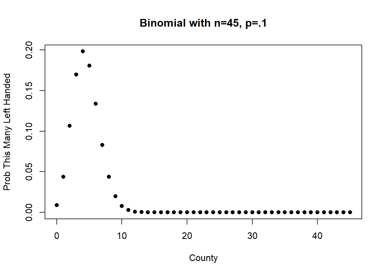
The expected value of this Binomial RV is \(n\pi=45*.1=4.5\), and accordingly, the highest values in the PMF are 4 & 5.
What is the expected probability of having 8 left handed presidents?
dbinom(8, 45, .1)
#> [1] 0.04370462
Just 4.3% of the time would we expect there to be exactly 8 left handed Presidents if Presidents were just a random draw from the population.
However, that wasn’t the question that I asked. I asked: what is the probability of having at least 8 presidents. That means I want to know the probability of having 8,9,10,11,12…. all the way up to 45 left handed presidents. We will see in coming weeks that this is relevant question to ask when we want to know the relative likelihood of rare events when judged against a distribution. The concept being: if Presidents are really being generated by this distribution, what is the probability we see something this extreme or more extreme? But regardless, how can we answer this question?
We can use the CDF instead:
plot(0:45,pbinom(0:45, 45, .1), xlab="County", ylab="Cumlative Prob This Many Left Handed",
main="Binomial with n=45, p=.1", pch=16)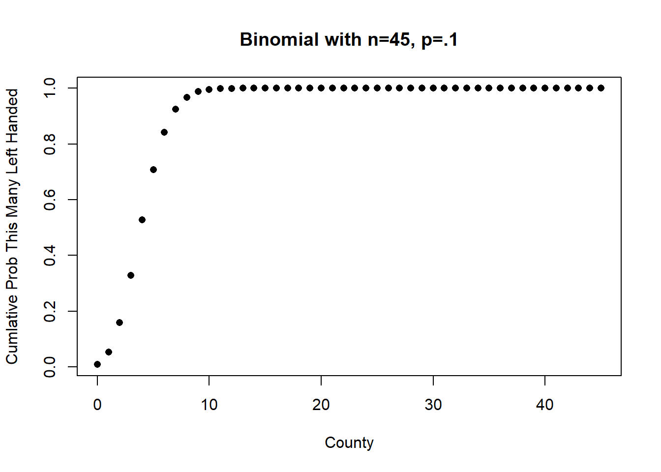 To think about how to use the
 pbinom() command to get the cumulative probability of 8,9,10,11,12… etc, it’s helpful to think about how it works. Here is the PMF and CDF for n=3 and \(\pi\)=.5). Looking just at the PMF, what is the cumulative probability of getting 2 or greater successes in 3 trials? That is \(.375+.125=.5\). It is tempting to assume that 1-pbinom(2,3,.5) would give us the right answer here, but it clearly wouldn’t (it would only give us .125). The pbinom() function gives us the probability that the cumulative probability is equal to or less than the value we give it, but if we subtract that from 1 we are subtracting out the probability that the binomial takes on the exact value we are giving it.
cbind(0:3,dbinom(0:3, 3, .5),pbinom(0:3,3,.5))
#>      [,1]  [,2]  [,3]
#> [1,]    0 0.125 0.125
#> [2,]    1 0.375 0.500
#> [3,]    2 0.375 0.875
#> [4,]    3 0.125 1.000
To get around this we must instead estimate probability that the binomial is less than or equal to 7. If we subtract this from 1 we get the probability that the binomial is greater than 7 (which includes 8, but not 7)!
1-pbinom(7,45,.1)
#> [1] 0.07569864
Since WWII, however, 6 out of 14 presidents have been left handed. What is the probability of at least 6 out of 14 presidents being left handed?
Altering our formula we get:
plot(0:14,dbinom(0:14, 14, .1), xlab="County", ylab="Prob This Many Left Handed",
     main="Binomial with n=45, p=.1", pch=16)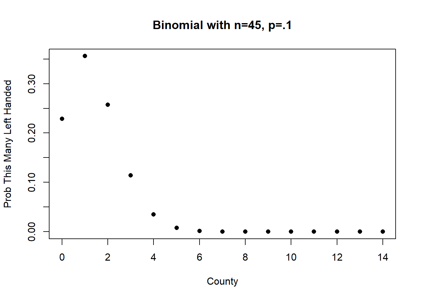
1-pbinom(5,14,.1)
#> [1] 0.001474054
Less than a 1% of something at least that extreme occurring by random chance. Seriously what is up with this??
We can use similar tools to investigate the uniform distribution.
Using our running example of a uniform variable representing the moment in the year you are born that ranges from 0 to 365 (this should have always been 0 to 365 I don’t know what I was thinking last time) : what is the probability of being born at exactly midnight at the start of the 345th day of the year?
Now you might think: this is a trick question, the answer is 0! And you are right! The answer is 0!
That being said, R will give you an answer to this.
dunif(345, min=0, max=365)
#> [1] 0.002739726
This is just the value of the PDF at that point. And as we saw the PDF for a uniform between the minimum and maximum values is equal to \(\frac{1}{b-a}=\frac{1}{365-0}=.002\). So R will give you an answer, even though the technically correct answer is 0.
A question that has a real answer, however, is what is the probability of being born before the 300th day of the year. Again we can use the CDF function here to calculate:
punif(300,0,365)
#> [1] 0.8219178
There is an 82% likelyhood of being born before the 300th day in the year.
What about the probability of being born in the last 15 days of the year?
Is this given by:
1- punif(350,0,365)
#> [1] 0.04109589
Yes! It is! Why don’t we have to adjust this down to, say, 349? That was only the case in the discrete random variable world because the probability of exactly the number we were giving was a real thing, and not taking that into account threw us off. Here the probability of exactly 350 is 0, so we don’t need to make any adjustments to this.
Next question: What is the probability of being born \(\pm 1 s.d.\) around the expected value of this uniform distribution?
Is the answer 68%? No! that only applies to the normal distribution.
The expected value of this uniform distribution is: \(E[X] = \frac{a+b}{2} = \frac{365}{2}= 182.5\)
The variance of a uniform is: \(V[X] = \frac{1}{12}(b-a)^2 = \frac{1}{12}(365)^2 = 11102.08\).
And therefore the standard error is \(\sqrt{11102.08}=105.36\).
Note that we could also have done \(\frac{1}{\sqrt{12}}(a-b) = \frac{1}{3.46}*365=105.36\)
Now to get this total probability around the mean, we can rely that the uniform is also symmetrical around the mean:
1- 2*punif(182.5-105.36, 0 , 365)
#> [1] 0.5773151
Around 58% of birth moments are within one standard deviation of the mean.
Finally some normal distribution questions:
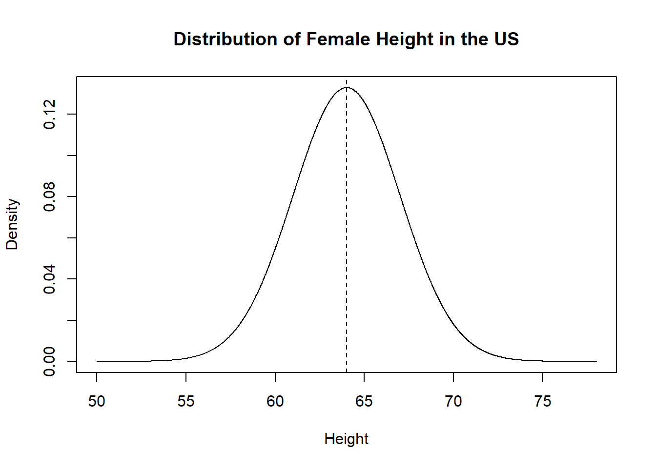
So we’ve seen already female height is normally distributed with a mean of 64 and a standard deviation of 3.
From that here is the PDF:
x <- seq(50,78, .01)
y <- dnorm(x, mean=64, sd=3)
plot(x, y, type="l", xlab="Height", ylab="Density", main="Distribution of Female Height in the US")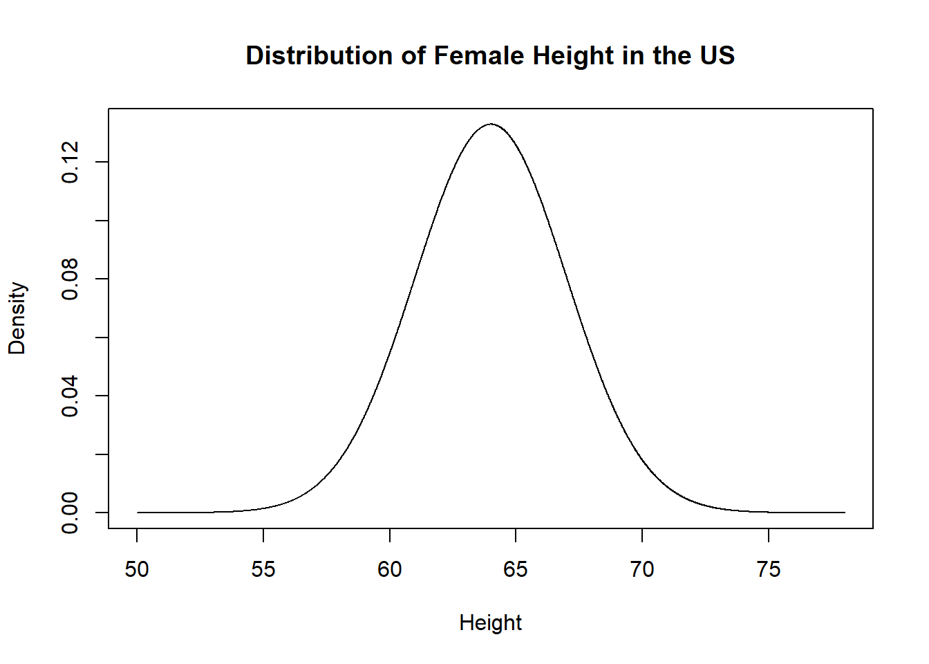
Let’s try to answer two classes of questions with the normal distribution:
For a given value of our variable, X, what percentage of the distribution is to the right or left of that value?
What is the value of X that puts a given percentage of the distribution to the right or left of that value?
The first question we’ve already seen above. We should be able to anser, for example: What proportion of women are expected to be under 5 feet tall (that’s to the left), and what proportion are expected to be over 5 feet tall (that’s to the right)?
plot(x, y, type="l", xlab="Height", ylab="Density", main="Distribution of Female Height in the US", lwd=2)
polygon(c(rev(x[x<=60]), min(x), 60), c(rev(y[x<=60]), 0, 0), col="dodgerblue")
abline(v=60, lty=2, lwd=2)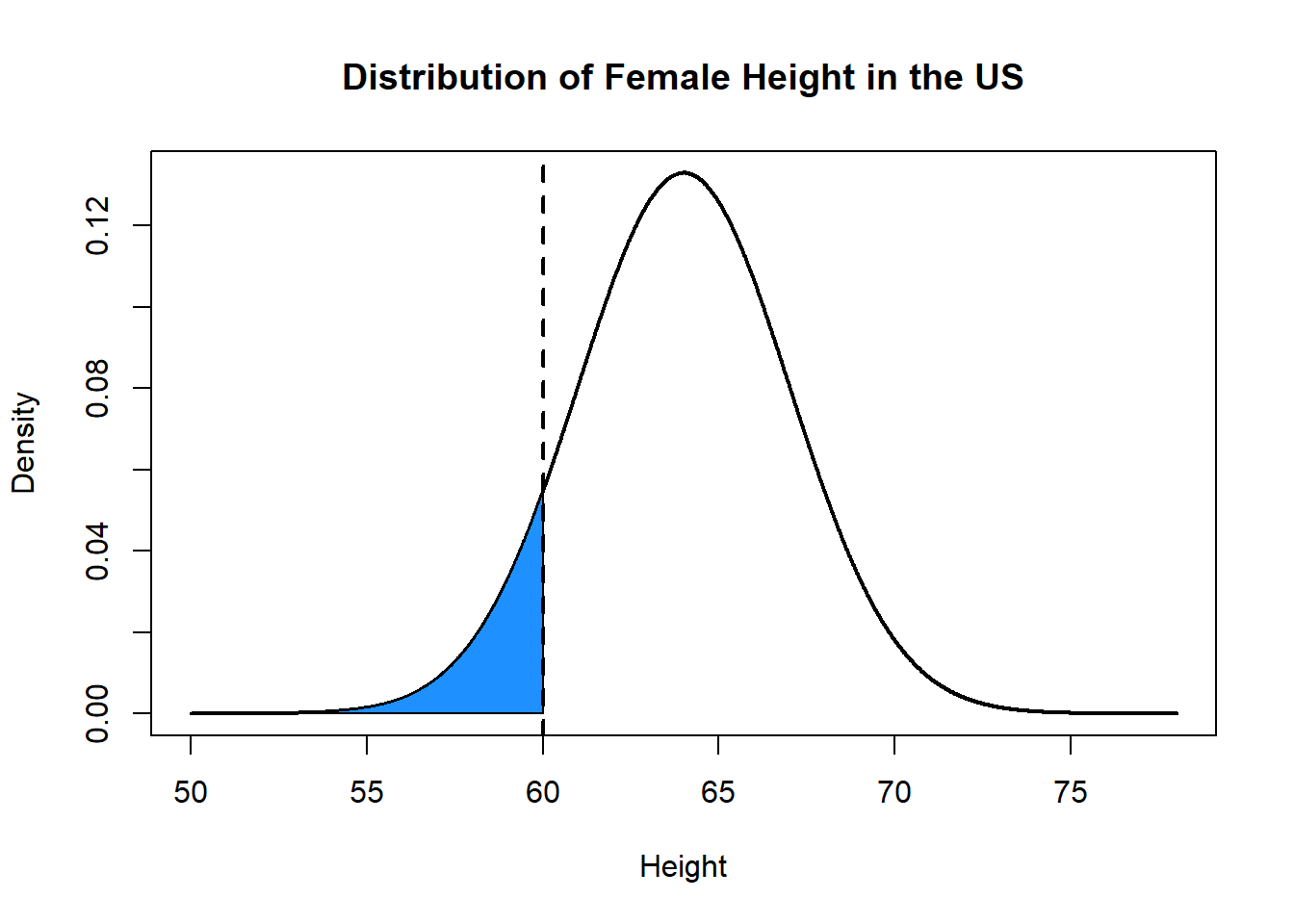
pnorm(60, mean=64, sd=3)
#> [1] 0.09121122
How can we calculate the inverse?
plot(x, y, type="l", xlab="Height", ylab="Density", main="Distribution of Female Height in the US", lwd=2)
polygon(c(x[x>=60], max(x), 60), c(y[x>=60], 0, 0), col="firebrick")
abline(v=60, lty=2, lwd=2)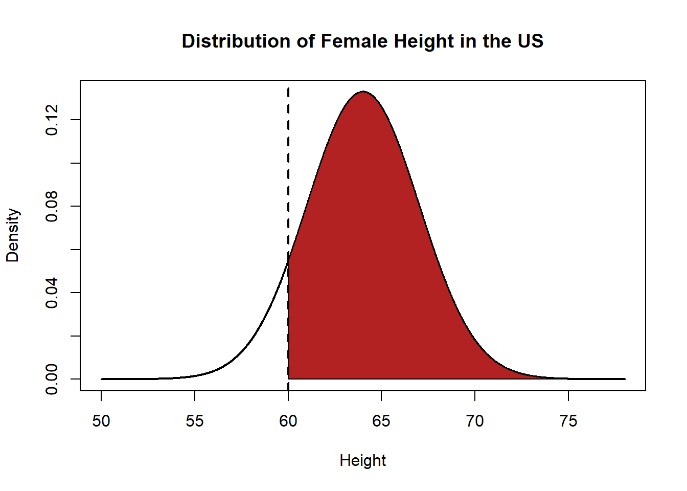
Well we know already that we can take 1 minus this value to get the inverse.
1-pnorm(60, mean=64, sd=3)
#> [1] 0.9087888
But there is also a shortcut to this answer. You may have noticed in the options to many of these pnorm commands that a default is lower.tail=T. By default, the CDF function gives us the probability of our random variable being less than or equal to the value that we specify. What happens if we turn lower tail to false?
pnorm(60, mean=64, sd=3, lower.tail=F)
#> [1] 0.9087888
It gives us the inverse automatically! In other words we can get the inverted CDF automatically by playing with this option.
What percentage of women are between 5 feet (60 inches) and 5 feet 8 inches (68 inches) tall?
plot(x, y, type="l", xlab="Height", ylab="Density", main="Distribution of Female Height in the US", lwd=2)
abline(v=60, lty=2, lwd=2)
abline(v=68, lty=2, lwd=2)
polygon(c(x[x>=60 & x<=68], 68, 60), c(y[x>=60 & x<=68], 0, 0), col="purple")
What percentage of women are between 5 feet (60 inches) and 5 feet 8 inches (68 inches) tall?
Two methods to think through this one. First we can think about overlapping areas:
plot(x, y, type="l", xlab="Height", ylab="Density", main="Distribution of Female Height in the US", lwd=2)
abline(v=60, lty=2, lwd=2)
abline(v=68, lty=2, lwd=2)
polygon(c(rev(x[x<=68]), min(x), 68), c(rev(y[x<=68]), 0, 0), col="firebrick")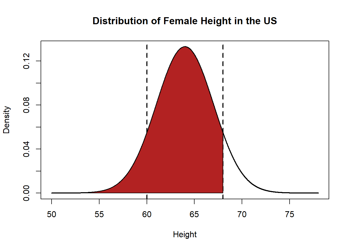
plot(x, y, type="l", xlab="Height", ylab="Density", main="Distribution of Female Height in the US", lwd=2)
abline(v=60, lty=2, lwd=2)
abline(v=68, lty=2, lwd=2)
polygon(c(rev(x[x<=60]), min(x), 60), c(rev(y[x<=60]), 0, 0), col="dodgerblue")
Red area minus blue area:
Or take advantage of symmetry:
plot(x, y, type="l", xlab="Height", ylab="Density", main="Distribution of Female Height in the US", lwd=2)
abline(v=60, lty=2, lwd=2)
abline(v=68, lty=2, lwd=2)
polygon(c(rev(x[x<=60]), min(x), 60), c(rev(y[x<=60]), 0, 0), col="dodgerblue")
polygon(c(x[x>=68], max(x), 68), c(y[x>=68], 0, 0), col="dodgerblue")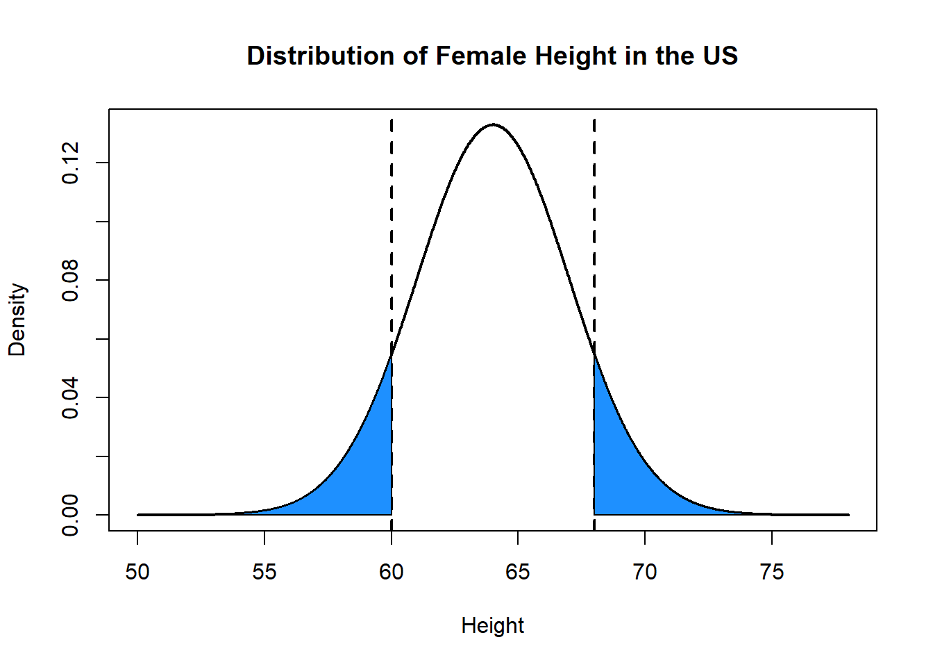
1-2*pnorm(60, mean=64, sd=3, lower.tail=T)
#> [1] 0.8175776
What percentage of women are within one standard deviation of the mean height?
pnorm(67, mean=64, sd=3, lower.tail=T) - pnorm(61, mean=64, sd=3, lower.tail=T)
#> [1] 0.6826895

1-2*pnorm(61, mean=64, sd=3, lower.tail=T)
#> [1] 0.6826895
But what if we want to know the opposite: how can we learn the value of our variable (again, in this case, height) that puts to its left or right a certain amount of probability?
What height does a woman have to be such that she is taller than 80% of women?
The way that we answer this this is with the “qnorm()” function. qnorm is the exact opposite of pnorm. While pnorm takes a value for our variable and spits out a percentage in one of the tails, qnorm takes a probability and tells you the value for the variable that puts that amount of probability in the the tail that you specify.
What height does a woman have to be such that she is taller than 80% of women?
qnorm(.8, mean=64, sd=3, lower.tail=T)
#> [1] 66.52486
plot(x, y, type="l", xlab="Height", ylab="Density", main="Distribution of Female Height in the US", lwd=2)
abline(v=66.5, lty=2, lwd=2)
polygon(c(rev(x[x<=66.5]), min(x), 66.5), c(rev(y[x<=66.5]), 0, 0), col="dodgerblue")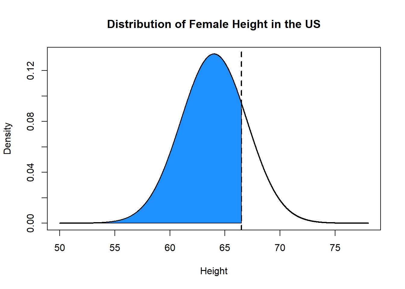
What question does this command answer?
qnorm(.8, mean=64, sd=3, lower.tail=F)
#> [1] 61.47514
This spits out 61.47: this is the height a woman has to be such that 80% of women are taller than her. The value of height that puts 80% of the probability mass to its right is 61.5.
plot(x, y, type="l", xlab="Height", ylab="Density", main="Distribution of Female Height in the US", lwd=2)
polygon(c(x[x>=61.47], max(x), 61.47), c(y[x>=61.47], 0, 0), col="firebrick")
abline(v=61.47, lty=2, lwd=2)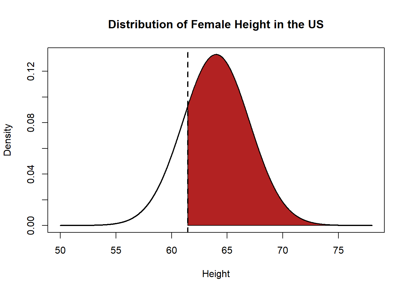
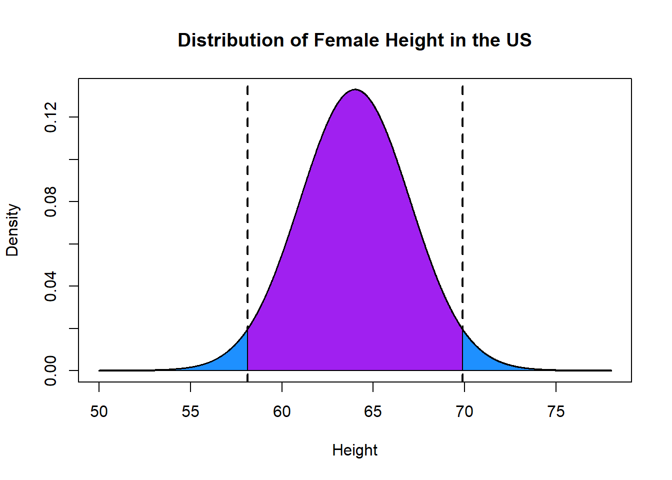
What are the two values of height that are equally on each side of the mean and define an area that contains 95% of all women?
Turn around the question: If we know the values that put 2.5% of the probability space in the left tail, and 2.5% of the probability in the right tail, then by definition there is 95% left in the middle.
qnorm(.025, mean=64, sd=3, lower.tail=F)
#> [1] 69.87989
qnorm(.025, mean=64, sd=3, lower.tail=T)
#> [1] 58.12011
plot(x, y, type="l", xlab="Height", ylab="Density", main="Distribution of Female Height in the US", lwd=2)
abline(v=58.12, lty=2, lwd=2)
abline(v=69.87, lty=2, lwd=2)
polygon(c(rev(x[x<=58.12]), min(x), 58.12), c(rev(y[x<=58.12]), 0, 0), col="dodgerblue")
polygon(c(x[x>=69.87], max(x), 69.87), c(y[x>=69.87], 0, 0), col="dodgerblue")
polygon(c(x[x>=58.12 & x<=69.87], 69.87, 58.12), c(y[x>=58.12 & x<=69.87], 0, 0), col="purple")