1 Introduction
This course focuses on the concept of inferential statistics.
At some point in learning about statistics or data science you may have heard instructors talk about samples and the population. The purpose of this class is to think a lot between the relationships between these two things and to focus our minds on the idea that this interplay is actually what the whole enterprise is all about.
What defines statistics is making conclusions about populations from a sample of data. (We infer things about populations from samples, hence the title of the class.)
“Population” is a pretty vague term however, and it encompasses a really wide range of things.
Sometimes what we mean is very obvious: In politics we often take random samples of a few thousand people to help us to understand the opinions and attitudes of the entire United States. In this case it’s quite clear that the sample is the random sample of people while the population is the adult public of the United States.
But lots of other things in our day-to-day lives are “samples” from some population, we often just don’t consider them as such.
For example: we might be interested in learning about the revenue potential of a small business, and have a few months of their finances as data. The goal is to use this sample of data (which may or may not be perfectly representative!) to better understand what the true earning potential of that business is. In this case the “population” is simply the true earning potential of the business.
If you are sports inclined we can think of the performance of a baseball hitter over a certain stretch of time as a “Sample” from the population that is their true hitting potential.
If it’s helpful (it is for me sometimes) we can re-frame the “population” as the “data generating process”. In the baseball example there is an underlying truth (the hitter’s true skill) which generates data (if the player hits the ball or not) when they step up to the plate.
In statistics, we look to make probabilistic inferences from samples about unknowable truths about the world. We will never precisely know the earning potential of a business, or how many Americans support a presidential candidate, or what level of hitting skill a baseball player has. We can, however, form estimates from a sample of data and estimate our level of uncertainty about the degree to which our answer represents the truth.
Here is a motivating example:
To start, we will use the 2020 National Election Study (NES), which interviewed just over 8000 Americans in the run up to the 2020 election.
A type of question often asked in survey’s like these is a “feeling thermometer” where individuals are asked to rate certain groups of politicians on a scale from 0 to 100, where 0 means the respondents feels “cool” towards the object, and 100 means the respondent feels “warm”.
This is how this looks in the first six rows of the data, focusing on the feeling thermometers for Trump and Biden. The first individual rated Trump at 100 and Biden at 0; the second individual rated both candidates at 0; the third rated Trump at 0 and Biden at 65 – and so on as we go down the rows.
library(rio)
anes <- import(file="https://raw.githubusercontent.com/marctrussler/IIS-Data/main/ANES2020Clean.csv")
#Examine the first 6 rows of data for these variables
head(anes[c("therm.trump","therm.biden")])
#>   therm.trump therm.biden
#> 1         100           0
#> 2           0           0
#> 3           0          65
#> 4          15          70
#> 5          85          15
#> 6           0          85
You likely have some skills already that may help you to summarize what this sample of data looks like. You have likely learned in previous classes all manner of methods to describe a dataset. For example, we can look at the distribution of responses to the feeling thermometer question for President Trump, represented as a density plot (which we can think of as a histogram for a continuous variable).
#Plot the density of the Trump feeling thermometer
plot(density(anes$therm.trump,na.rm=T), xlim=c(0,100), main="Distribution of Trump Themometer Ratings")
abline(v=mean(anes$therm.trump,na.rm=T), lty=2)
legend("topright", c(paste("Mean = ",round(mean(anes$therm.trump,na.rm=T),2 )),
                     paste("SD = ",round(sd(anes$therm.trump,na.rm=T),2 )) ), lty=2, col=c("Black", "White"))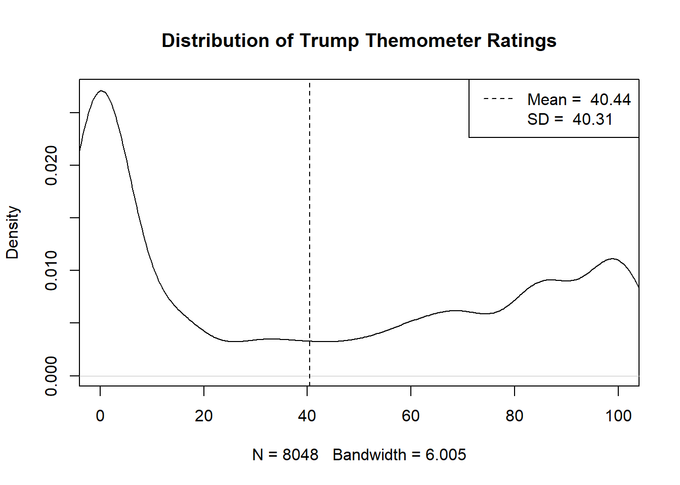
We can see that in our data there is a lot of density around 0, and a lot of density from 80 to 100. What does this mean? This means that in our sample there are a lot of individuals who do not like Donald Trump (give him a rating of 0) and a lot of individuals who have a fairly warm view of Donald Trump (give him a rating near 100). With very few answers around 50, not many individuals have ambivalent feelings towards the former President.
We can also summarize the distribution of this variable in the sample with summary statistics. The mean – or simple average – of this variable, for example, is 40.44. The standard deviation – which can be thought of as how much each individual deviates from the mean, on average – is 40.31.
The problem is, that’s not at all what we care about. What we care about, in the example of a Trump feeling thermometer, is how all voters in the feel about Trump, not just the ones in this sample. What is the true average feeling towards Trump amongst all voters? How spread out is that opinion? Do the opinions of Democrats and Republicans differ? All of these questions are not immediately or obviously answered by the data in front of us.
It is tempting to say: well if this is a sample of data from the population isn’t the answer the same in the population? Isn’t it good enough to get a sample, report what’s in that sample, and assume it’s the same as the population?
To some degree our answer to this is actually, yes! But let’s think for a little bit: if we took another sample of 8000 Americans would this plot look exactly the same? How much could we expect it to vary? It obviously will not be exactly the same…. so how do we know that this distribution is the one that is representative of the population?
Let’s return to the baseball example to further think about this. I talked before about how a series of at-bats is a “sample” of the population (or Data Generating Process) which is the hitters true batting ability.
Pretend we know that a batter’s true ability is that they get a hit in 35% of at-bats (a .350 batting average). The following code simulates 10000 at bats for this batter. Don’t worry about the nature of this code right now.
We can ask the question: for any given run of 20 at-bats (about 4 games worth), is a sample a good representation of the hitters true ability? Afterall, 4 baseball games is a lot of baseball! You should be able to determine whether someone is a good or bad hitter in that time.
#Use a loop to calculate the moving 20-at-bat batting average for this batter
moving.average <- NA

for(i in 1:9981){
 moving.average[i] <-  mean(hits[i:(i+19)])
}

plot(1:500, moving.average[1:500], type="l", axes=F,
     xlab="", ylab="Batting Average for Previous 20 Games", cex=.5)
abline(h=.35, lty=2)
axis(side=2, las=2)
axis(side=1)
Sometimes the batter is right on .350, but they are often not. Indeed, there are 4 game stretches where the batter is hitting .100, and 4 game stretches where they are hitting .600, just by random chance.
So not every sample is a sample that is representative of the population, so we can’t just rely on “Well the population is unknowable but I have a sample so it’s fine!”.
Here’s another example from real data. We can go further in terms of the feeling thermometer and look at the relationship between age and feelings towards Trump. Here are those data represented in a scatterplot:
#Plot Feeling Thermometer against age
plot(anes$age, anes$therm.trump)
abline(lm(anes$therm.trump ~ anes$age), col="firebrick", lwd=2)
These raw data are a bit harder to parse. Individuals are likely to anchor to certain responses when using the feeling thermometer (0,10,20 etc.) so there is not continuous variation on the y-axis. Further, people at each age have a wide variety of opinions about Trump: there are 20 year olds that love him, and 20 year olds that hate him; there are 80 year olds3 that love him, and 80 year olds that hate him.
So how can we describe these data? The method that we will focus on in this class is Ordinary Least Squares (OLS) regression. The red line in the figure represents the OLS estimate for the line that best represents these data. We can further use R to describe this line:
#Run a regression predicing feelings towards Trump by age
m <- lm(therm.trump ~ age, data=anes)
summary(m)
#>
#> Call:
#> lm(formula = therm.trump ~ age, data = anes)
#>
#> Residuals:
#>    Min     1Q Median     3Q    Max
#> -47.15 -38.13 -11.79  41.26  67.97
#>
#> Coefficients:
#>             Estimate Std. Error t value Pr(>|t|)
#> (Intercept) 27.64585    1.43952  19.205   <2e-16 ***
#> age          0.24380    0.02661   9.162   <2e-16 ***
#> ---
#> Signif. codes:
#> 0 '***' 0.001 '**' 0.01 '*' 0.05 '.' 0.1 ' ' 1
#>
#> Residual standard error: 40.11 on 7725 degrees of freedom
#>   (553 observations deleted due to missingness)
#> Multiple R-squared:  0.01075,    Adjusted R-squared:  0.01062
#> F-statistic: 83.95 on 1 and 7725 DF,  p-value: < 2.2e-16
We will learn a lot about what each of these numbers mean, but in short here is what this is telling us. The red line above has a y-intercept of 27.64. This means that when age is 0 (not possible!) the average feeling towards Trump is 27.64. The slope of the line is .24. This means that as age increases by one year the Trump thermometer increases by .24 units. In other words, in these data there is a positive relationship between age and feelings towards Trump. Which checks out given what we know about politics.
But once again, we have a pretty limited interest in describing what is happening in these data in particular. Our real object of interest is the degree to which age and feelings towards Trump are related in the population. If we look at the row for the variable age, the rest of that information is what allows us to understand what this relationship is in the whole population. Things like the “Standard Error”, “T-Value”, and “p-score” are all ways in which we come to understand our ability to make inferences about the whole population based on the information contained in this one sample.
How is that possible? How can we possibly learn something about all the eligible voters in the United States from a sample of a few thousand people? The reason will be explained in detail throughout the course, but the basic intuition is described briefly here. Statisticians have determined that if you were to run the same survey again, and again, and again, hundreds-of-thousands of times; and in each sample record an estimate of interest (such as the mean, or a regression coefficient), the resulting distribution of estimates is extremely predictable.
Here is a quick simulation of what that looks like. All of the code below will make a lot more sense as the class goes on. Try not to focus for the code for now, just the intuition that it is giving.
We can use R to create fake data on which we can run a regression:
#Creation of fake data:
set.seed(19104)
x.prime <- rnorm(1000,mean=3, sd=6)
y.prime <- 3*rnorm(1000) + 4*x.prime + rnorm(1000, 0, 30)
plot(x.prime,y.prime)
abline(lm(y.prime ~ x.prime), col="firebrick", lwd=2)
summary(lm(y.prime~x.prime))
#>
#> Call:
#> lm(formula = y.prime ~ x.prime)
#>
#> Residuals:
#>     Min      1Q  Median      3Q     Max
#> -87.604 -18.997  -0.583  19.131  93.628
#>
#> Coefficients:
#>             Estimate Std. Error t value Pr(>|t|)
#> (Intercept)   0.2532     1.0607   0.239    0.811
#> x.prime       3.8715     0.1557  24.858   <2e-16 ***
#> ---
#> Signif. codes:
#> 0 '***' 0.001 '**' 0.01 '*' 0.05 '.' 0.1 ' ' 1
#>
#> Residual standard error: 29.74 on 998 degrees of freedom
#> Multiple R-squared:  0.3824, Adjusted R-squared:  0.3818
#> F-statistic: 617.9 on 1 and 998 DF,  p-value: < 2.2e-16
Looking at the resulting data, there is a pretty clear positive relationship between these two variables, when x gets higher, we expect y to get higher. Looking at the output of the regression we see that the slope is around 4. This simply means, for these data, as x increases by one unit y increases by 4 units, on average.
Like the ANES data, we know that this is just one possible dataset of many datasets that we could have. Unlike the ANES data, here we know that the population/data generating process is, so we can just actually see what happens when we create new samples of 1000 and run the same regression. Here is one additional sample pulled from the exact same population. To make the point clear, the original data points and regression line are displayed in grey, and the new data and regression line are in orange.
x <- rnorm(1000,mean=3, sd=6)
y <- 3*rnorm(1000) + 4*x + rnorm(1000, 0, 30)
plot(x.prime,y.prime, col="gray80")
abline(lm(y.prime ~ x.prime), col="gray30", lwd=2)
points(x,y, col="darkorange")
abline(lm(y~x), col="darkorange", lwd=2)
summary(lm(y~x))
#>
#> Call:
#> lm(formula = y ~ x)
#>
#> Residuals:
#>      Min       1Q   Median       3Q      Max
#> -104.107  -21.801   -0.963   21.259   91.605
#>
#> Coefficients:
#>             Estimate Std. Error t value Pr(>|t|)
#> (Intercept)  -0.5727     1.1068  -0.517    0.605
#> x             3.6858     0.1651  22.329   <2e-16 ***
#> ---
#> Signif. codes:
#> 0 '***' 0.001 '**' 0.01 '*' 0.05 '.' 0.1 ' ' 1
#>
#> Residual standard error: 30.62 on 998 degrees of freedom
#> Multiple R-squared:  0.3331, Adjusted R-squared:  0.3325
#> F-statistic: 498.6 on 1 and 998 DF,  p-value: < 2.2e-16
We can see that the new orange data points are not identical to the grey data points. This is new data. But these new data still reveal the same underlying relationship. Because the data points are a little bit different, the regression line is also a little bit different. Looking at the output of the regression we can see that the slope coefficient is slightly different than what we got on with the first sample.
Now let’s go absolutely crazy. Let’s generate 5000 additional samples. That is, we are going to make 5000 independent samples of 1000 people. This is similar to if we re-ran the ANES 5000 times. I’m going to re-sample from this population 5000 times. Each time I’m going to run the regression we have run on the new data and save the slope coefficient.
coefs <- rep(NA, 5000)

plot(x.prime,y.prime, type="n")
abline(lm(y.prime ~ x.prime), col="gray30", lwd=2)
for(i in 1:5000){
x <- rnorm(1000,mean=3, sd=6)
y <- 3*rnorm(1000) + 4*x + rnorm(1000, 0, 30)
m <- lm(y ~ x)
coefs[i] <- coefficients(m)["x"]
abline(m, col="gray60")
}
abline(lm(y.prime ~ x.prime), col="firebrick", lwd=2)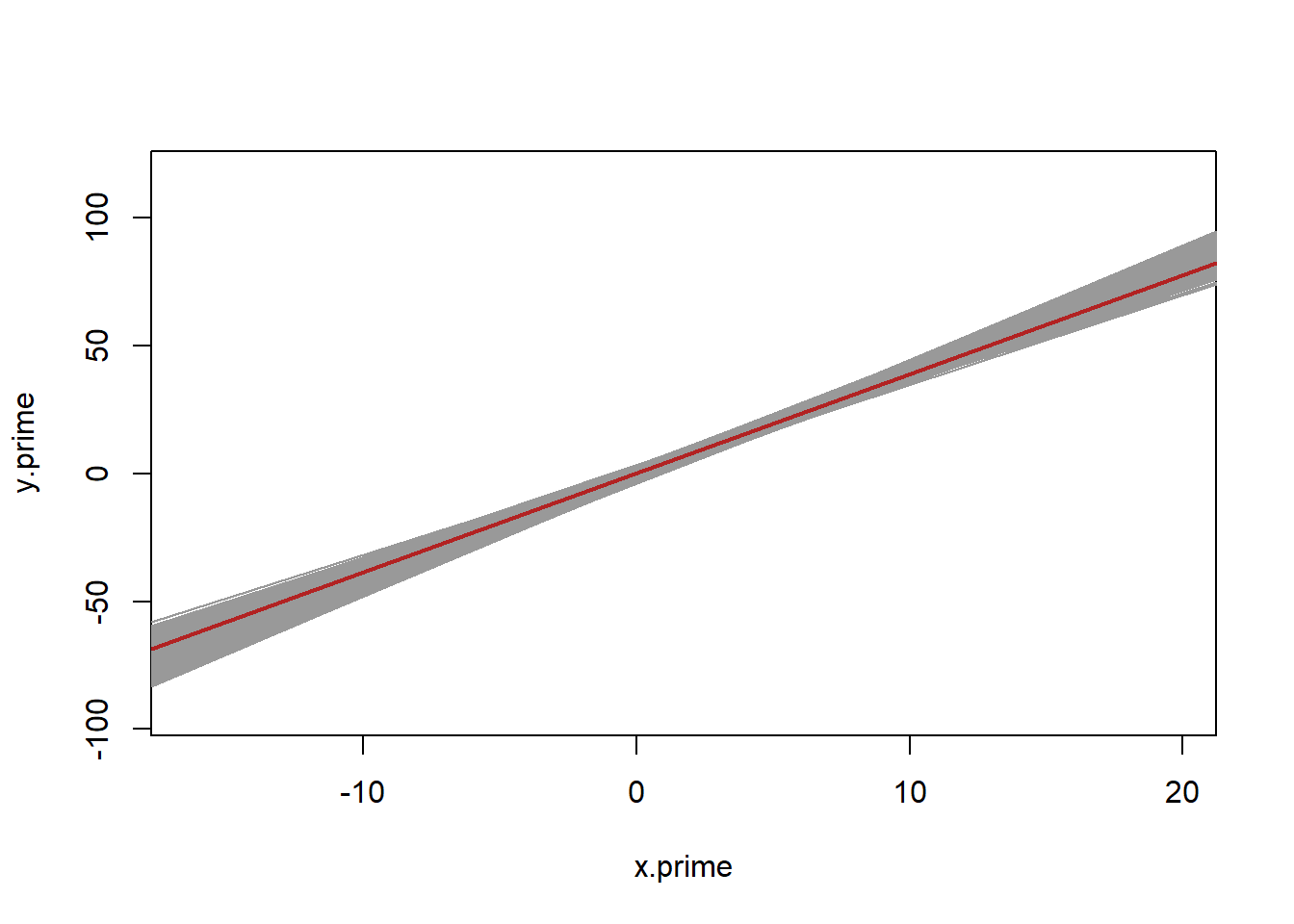
Displayed in grey is 5000 different regression lines from 5000 different samples all stacked on top of one another. They are all a little bit different but all speak to the relationship in the population.
What does the distribution of these coefficients look like? To understand that we can use a density plot. A density plot is like a continuous histogram. The x-axis shows all the posisble values a particular variable and the y-axis shows how common those value are. Here is what the density plot of all the coefficients from our 5000 samples looks like:
plot(density(coefs), main="Sampling Distribution of Beta Coefficients")
abline(v=4, col="firebrick", lwd=2)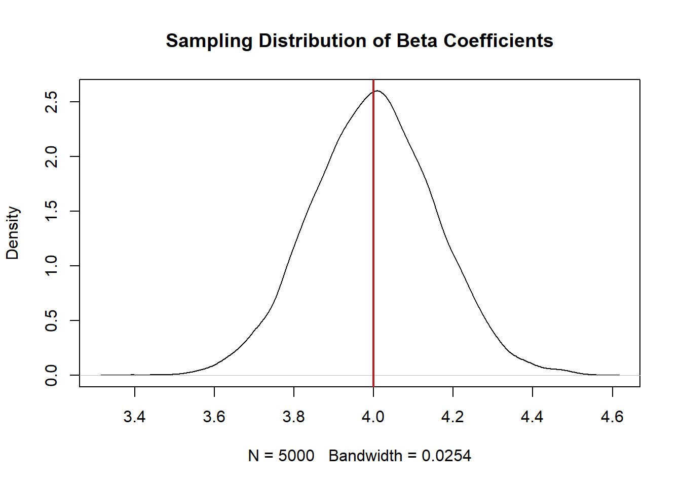
The distribution of these 5000 coefficients, which we will come to learn is called the sampling distribution is a bell curve. Indeed, it is actually a special type of bell curve called the normal distribution (which I’m sure you’ve heard about).
So to summarize: if we have the ability to magically re-sample the same population many times, and each time calculate some statistic (here, a regression coefficient) we get a normal distribution of coefficients.
Here is the magic/mind-bending part of this. Let’s look again at the very first regression result from the very first sample:
summary(lm(y.prime ~ x.prime))
#>
#> Call:
#> lm(formula = y.prime ~ x.prime)
#>
#> Residuals:
#>     Min      1Q  Median      3Q     Max
#> -87.604 -18.997  -0.583  19.131  93.628
#>
#> Coefficients:
#>             Estimate Std. Error t value Pr(>|t|)
#> (Intercept)   0.2532     1.0607   0.239    0.811
#> x.prime       3.8715     0.1557  24.858   <2e-16 ***
#> ---
#> Signif. codes:
#> 0 '***' 0.001 '**' 0.01 '*' 0.05 '.' 0.1 ' ' 1
#>
#> Residual standard error: 29.74 on 998 degrees of freedom
#> Multiple R-squared:  0.3824, Adjusted R-squared:  0.3818
#> F-statistic: 617.9 on 1 and 998 DF,  p-value: < 2.2e-16
Looking at the line for x.prime we see something called the “Std. Error”. What is truly magic is that this number contains all the information that we need to determine what the sampling distribution woulld looke like if we generated 5000 (or really, an infinite number of samples).
To prove it, I can use R to draw a normal distribution on top of our sampling distribution using only information from that first regression table:
plot(density(coefs), main="Sampling Distribution of Beta Coefficients")
x <- seq(3,5,.001)
#Note the use of  0.1557, which is from the regression table above!
points(x,dnorm(x, mean=4, sd= 0.1557), type="l", col="darkorange")

abline(v=4, col="firebrick", lwd=2)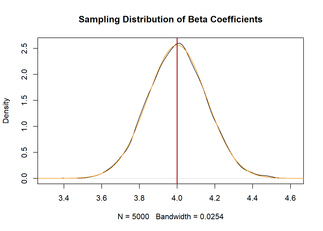
The distribution is identical. Let me repeat what’s happening here. The black line is the distribution of 5000 regression coefficients. In the real world, we can’t just generate 5000 regression coefficients! The orange line is what we predict this sampling distribution will look like based on the results of one sample. In other words: we don’t have to do things 5000 times! We get the distribution from just one sample!
Because we can guess with a great deal of accuracy what this distribution of statistics from repeated sampling would be, we are able to determine how likely or unlikely the result we achieved is under different scenarios (what we call null hypothesis testing). We will learn that the most critical question asked by statistics is: if there is nothing going on here, if there is no relationship in the population, how likely is it to get the result I am seeing in my sample?
If this is all gobblygook right now, do not worry! The big thing to take away from this introduction is the following: the goal of statistics is to understand the population, not to simply describe the sample we have in front of us. To gain insight on this, we imagine calculating our statistic of interest many, many times. The resulting distribution is a knowable, calculable thing, which allows us to determine how special our statistic of interest is.