Problem Set 1
Problem Set Due Wednesday September 27th at 7pm on Canvas.
For this problem set you will hand in a .Rmd file and a knitted html output.
Please make life easy on us by using sections to clearly delineate questions and sub-questions.
Comments are not mandatory, but extra points will be given for answers that clearly explains what is happening and gives descriptions of the results of the various tests and functions.
Reminder: Put only your student number at the top of your assignment, as we will grade anonymously.
Collaboration on problem sets is permitted. Ultimately, however, the code and answers that you turn in must be your own creation. You can discuss coding strategies, code debugging, and theory with your classmates, but you should not share code or answers in any way.
Please write the names of any students you worked with at the top of each problem set.
Question 1: Probability & Counting
(a) In a game of poker each player is dealt 5 cards from a 52 card deck. How many different 5 card poker hands can be generated from a 52 card deck? (Hint: Is this a permutation or a combination?).
choose(52,5)
#> [1] 2598960
This is a combination because the order of poker hands doesn’t matter
(b) There are 4 suits in a card deck, each consisting of 13 cards. A “flush” is a poker hand where all 5 cards are of the same suit. Calculate the probability of being dealt a flush. (Hint: You first need to count all the ways you can make a 5 card hand using only cards from one suit.)
#How many ways can you have a flush within a suit of 13 cards?
choose(13,5)
#> [1] 1287

#There are 4 suits so
1287*4
#> [1] 5148

#Out of all possible hands
(choose(13,5)*4)/choose(52,5)
#> [1] 0.001980792
The odds of a flush are about .2%.
(c) Simulate the answer to question (b) using R. Run a loop 100000 times that draws 5 cards from a deck of 52, where there are 4 suits with 13 cards each. Note, that we don’t care which cards are which within a suit. We just need 13 hearts, 13 diamonds, 13 clubs, 13 spades. How often are you dealt a flush? (Hint: to see if all the cards in my hand were of the same suit I started with the unique() command.)
#Set up
deck<- c(rep("hearts",13),rep("diamonds",13), rep("clubs",13), rep("spades",13))

#Sample WITHOUT REPLACEMENT
hand <- sample(deck,5,replace=F)

#Test to see if all of the cards are from the same suit

length(unique(hand))==1
#> [1] FALSE

#No  they are not

#Loop and record successes:

flush <- rep(NA, 100000)

for(i in 1:length(flush)){
  hand <- sample(deck,5,replace=F)
  flush[i] <- length(unique(hand))==1
}
prop.table(table(flush))
#> flush
#>   FALSE    TRUE
#> 0.99797 0.00203
We get a approximarely similar .2% via simulation.
(d) A manufacturer of code-based locks comes to you worried that the codes on his lock are too easy to guess. He tells you that his locks have a dial with 10 numbers and the codes are 3 digits long. Like most locks, the numbers in the code cannot repeat and the order of the numbers matters. Calculate the probability of guessing this code using both math and simulation. For the simulation, run the loop 1 million times.
#A lock with 10 numbers and a code length of 3

#This gives the number of combinations:
choose(10,3)
#> [1] 120

#Need to multiply by 3! to get permutations
1/(choose(10,3)*factorial(3))
#> [1] 0.001388889

#The probability of guessing this lock is actually quite low at .014%

#Through simulation
set.seed(19104)
dial <- seq(1,10,1)
prime <- sample(dial,3, replace=F)
result <- rep(NA, 1000000)

for(i in 1:length(result)){
  result[i] <- all(sample(dial,3, replace=F)==prime)
}
prop.table(table(result))
#> result
#>    FALSE     TRUE
#> 0.998599 0.001401

#We get approximately the same result through simulation
Both the simulation and math routes give a similar answer that any given guess has a .01% probability of being correct.
(e) To help this manufacturer we want to determine if it’s more effective to manufacture a bigger dial or to require the user to use a longer code. Using R to simulate each possibility 1 million times, make two graphs. For the first graph, determine the probability of guessing a code with dial sizes from 10 to 30 numbers and a 3 digit code. For the second graph, determine the probability of guessing a code with a dial size of 10, but code lengths from 3-10 numbers long. What do you find?
#Reuse our code but make the dial length a variable
set.seed(19104)

lengths <- seq(10,30,1)
prob.guess <- rep(NA, length(lengths))

for(j in 1:length(lengths)){
  dial <- seq(1,lengths[j],1)
  prime <- sample(dial,3, replace=F)
  result <- rep(NA, 1000000)

  for(i in 1:length(result)){
    result[i] <- all(sample(dial,3, replace=F)==prime)
  }
 prob.guess[j] <- prop.table(table(result))[2]
}

plot(lengths, prob.guess, pch=16, type="b", ylab="Probability of Guessing Right",
     xlab="Dial Sizes",
     main="Probability of Correct Guess with Code Length 3 and Varying Dial Size")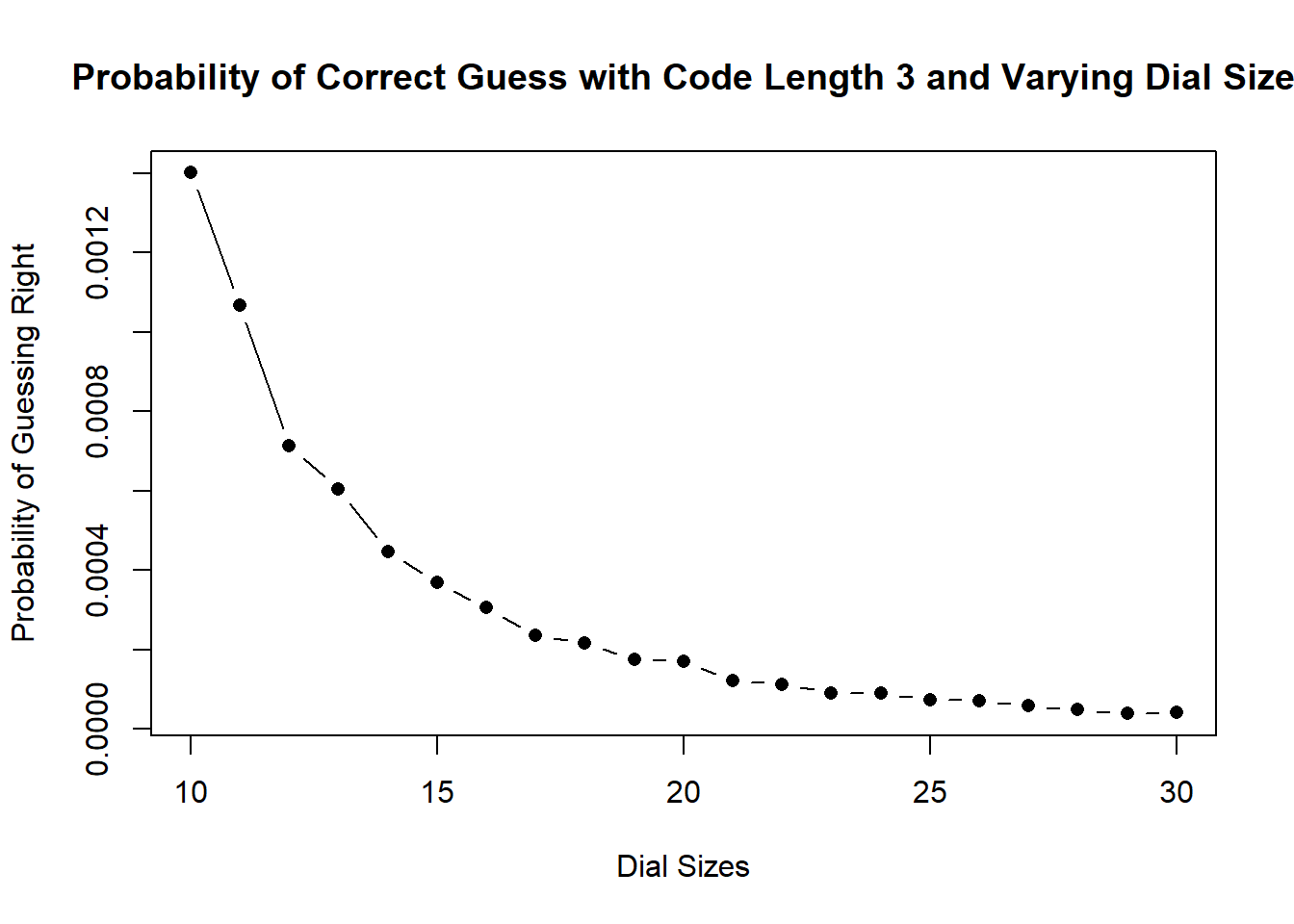
#Reuse our code but make the dial length a variable
set.seed(19104)

codes <- seq(3,10,1)
prob.guess <- rep(NA, length(codes))

for(j in 1:length(codes)){
  dial <- seq(1,10,1)
  prime <- sample(dial,codes[j], replace=F)
  result <- rep(NA, 1000000)

  for(i in 1:length(result)){
    result[i] <- all(sample(dial,codes[j], replace=F)==prime)
  }
 prob.guess[j] <- mean(result)
}

plot(codes, prob.guess, pch=16, type="b", ylab="Probability of Guessing Right", xlab="Code Length",
     main="Probability of Correct Guess with Dial Size 10 and Varying Code Length")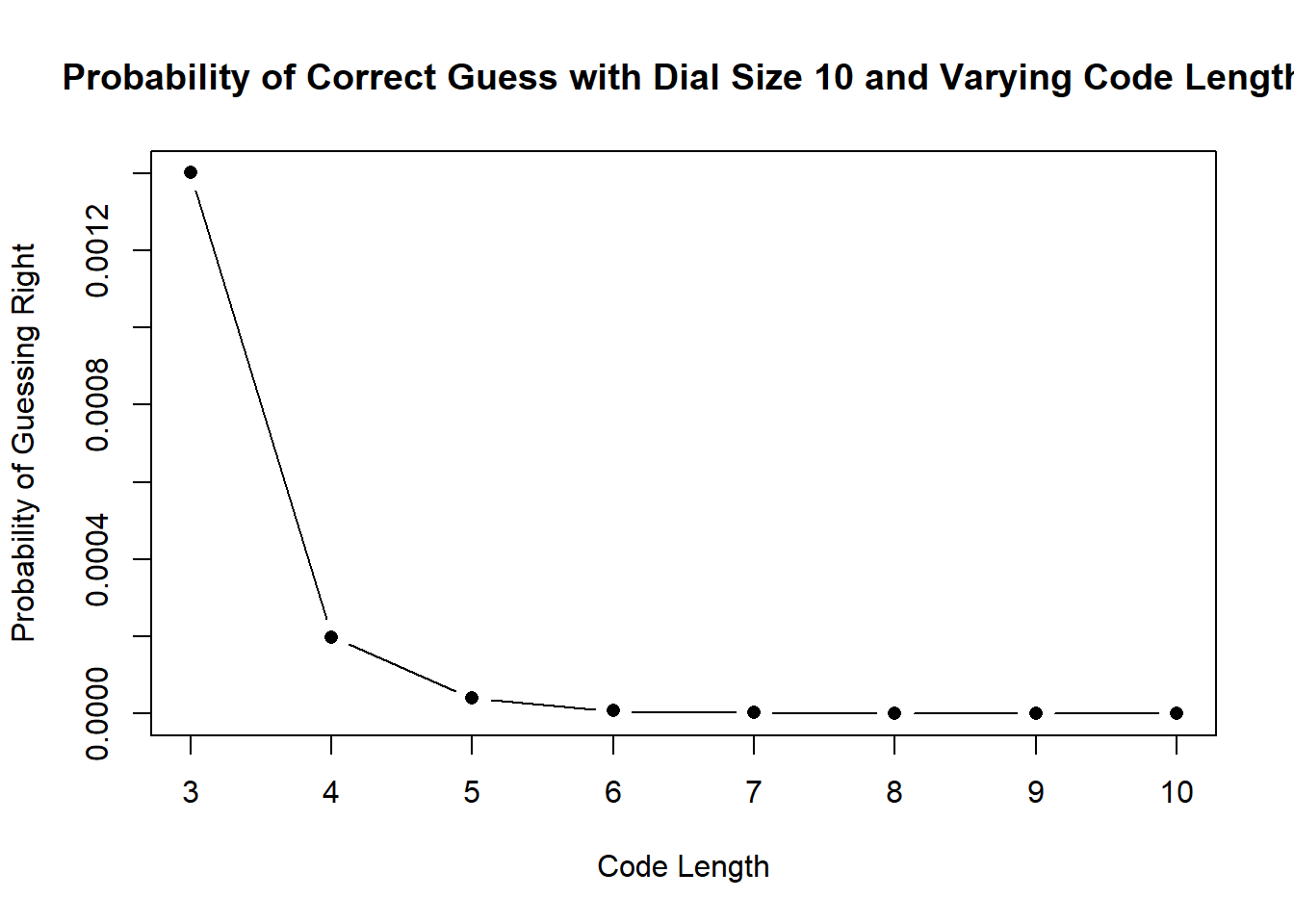
As would be expected, reducing both increasing the dial size and increasing the code length cause the probability of any particular combination being a correct guess to decrease. That being said, it appears that increasing the code length has a much more dramatic effect than increasing the dial size.
For example, with a code of length 3 increasing the dial size from 10 to 11 changes the number of permutations by:
While changing the code length from 3 to 4 for a dial length of 10 increases the number of permutations by:
Factorials, man!
Question 2: Conditional Probability in Data
This problem is going to have you examine some data on the outcomes of college basketball games. I have a theory for why in certain games that underdogs (i.e., the team that is seen as less likely to win a game before the game starts) will perform better than people expect when the score is higher than people expect, and favorites (i.e., the team that is seen as more likely to win a game before the game starts) will perform better than people expect when the score is lower than people expect. In other words, I believe that upsets are more likely in higher scoring games. To test this theory, I tracked the outcomes of 241 games between 1/22/2019-3/29/2019 in which I assessed my theory would apply. Data about these games are contained in ‘’CollegeBasketball.csv’’. We are going to examine these data to see whether the empirical evidence is consistent with my theory.
You can load the data via:
#Load the data
bball <- read.csv("https://raw.githubusercontent.com/marctrussler/IIS-Data/main/CollegeBasketball.csv")
Here is a description of the relevant variables contained in “CollegeBasketball.csv”:
-
PredictedDifferenceare gamblers’ expectations for how many more points the favorite will score compared to the underdog. Because the favorite is expected to win (they are the favorite!) this number is always positive. -
ActualDifferenceis how many more points the favorite scored than the underdog in the game, meaning that it is a negative number when the underdog won the game. -
PredictedPointsare gamblers’ expectations about the total number of points that will be scored in the game. -
ActualPointsis how many combined points the favorite and the underdog scored.
Answer the following questions using R:
(a) Make a new variable that is equal to ActualDifference minus PredictedDifference. Create a histogram (hist()) that shows the distribution of this variable and briefly describe what it shows.
#Compute Game Delta
bball$game.delta <- bball$ActualDifference - bball$PredictedDifference
#If this is 0 the predicted difference was exactly the same as the actual difference
#If this is positive, actual winners margin was larger than predicted winning margin: the favorite overperformed
#If this is negative, actual winners margin was smaller than predicted winning margin: the underdog overperformed

hist(bball$game.delta, main="Distribution of Game Delta",
     xlab="Actual Difference minus Predicted Difference for Favorite")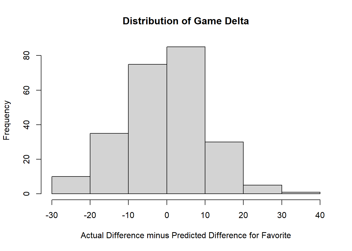
Slightly more outcomes are larger than 0, which suggests that more often the favorite over performs.
(b) Let \(W\) represent the event that the favorite won a basketball game by more points than expected, \(E\) represent the event that the favorite won a basketball game by exactly the number of points that were expected, and \(L\) be the event that the favorite won a basketball game by fewer points than expected or lost a basketball game. Using the variable you created in (a), make three new boolean variables indicating whether these events occurred in each game and use these variables to calculate within the sample \(P(W)\), \(P(E)\), and \(P(L)\).
#Actual greater than predicted means a positive delta:
bball$W <- bball$game.delta>0

#Actual equal to predicted means delta of 0
bball$E <- bball$game.delta==0

#Actual less than predicted means negative delta
bball$L <- bball$game.delta<0

#P(overperform)
mean(bball$W)
#> [1] 0.5020747
#P(on exp)
mean(bball$E)
#> [1] 0.02904564
#P(underperform)
mean(bball$L)
#> [1] 0.4688797
The probability that favorite overperforms is around 50%. The probability that the score ends exactly as predicted is around 3%, and the probability that the favorite underperforms is around 47%.
(c) Make a new variable that is equal to ActualPoints minus Predicted Points. Create a histogram that shows the distribution of this variable and briefly describe what you see.
#Compute points Delta
bball$points.delta <- bball$ActualPoints - bball$PredictedPoints
#If this is 0 the predicted points was exactly the same as the actual difference
#If this is positive, actual points margin was larger than predicted points: game was relatively high scoring
#If this is negative, actual points was smaller than predicted points: game was relatively low scoring

hist(bball$points.delta, main="Distribution of Total Points Delta",
     xlab="Actual Total Points minus Predicted Total Points")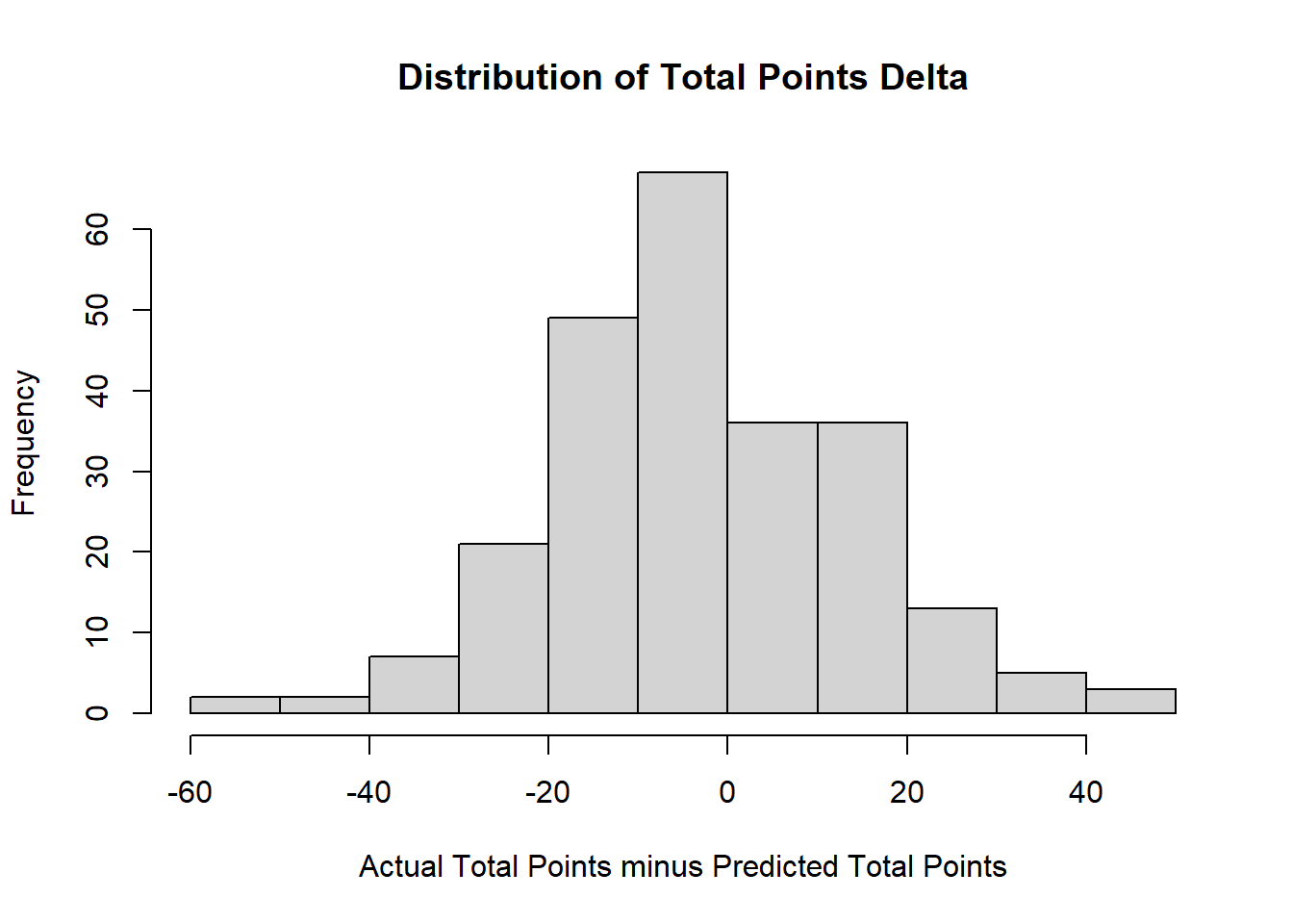
#Slightly more outcomes are smaller than 0, which suggests that more often the game is relatively low scoring compared to expectations.
(d) Let \(O\) represent the event that more combined points were scored than expected, \(T\) represent the event that the combined points scored were exactly the number expected, and \(U\) represent the event that fewer combined points were scored than expected. Make new variables indicating whether these events occurred in each game and use these variables to calculate within the sample \(P(O)\), \(P(T)\), and \(P(U)\).
#Actual greater than predicted means a negative delta:
bball$O <- bball$points.delta>0
#Equal
bball$T <- bball$points.delta==0
#Predicted greater than actual means positive delta
bball$U <- bball$points.delta<0

#P(overscore)
mean(bball$O)
#> [1] 0.3858921
#P(on exp)
mean(bball$T)
#> [1] 0.04149378
#P(underscore)
mean(bball$U)
#> [1] 0.5726141
Around 39% of the time more points are scored in the game then what was expected. Approximately 4% of the time the final score is exactly what was predicted (that’s weird). And approximately 57% of the time there are less points scored than expected.
(e) Using the conditional probability formula discussed in lecture, calculate within the sample \(P(W \mid U)\), \(P(L \mid U)\), \(P(W \mid O)\), \(P(L \mid O)\).
#Conditional probability is P(A|B) = P(A&B)/P(B)

#P(W|U), the probability of favorite overperformance in a low scoring game
mean(bball$W & bball$U)/mean(bball$U)
#> [1] 0.557971
#The probability of overperformance in a low scoreing game is 56%

#P(L|U), the probability of favorite underperformance in a low scoring game
mean(bball$L & bball$U)/mean(bball$U)
#> [1] 0.4057971
#The probability of overperformance in a low scoreing game is 40.5%


#P(W|O), the probability of favorite overperformance in a high scoring game
mean(bball$W & bball$O)/mean(bball$O)
#> [1] 0.4301075
#The probability of overperformance in a low scoreing game is 43%

#P(L|O), the probability of favorite underperformance in a high scoring game
mean(bball$L & bball$O)/mean(bball$O)
#> [1] 0.5483871
#The probability of overperformance in a low scoreing game is 54.9%
(f) In two or three sentences: what is your conclusion about my theory?
The theory is that favorites will be more likely to overperform in low scoring games and underperform in high scoring games.
This theory is borne out by the data.
Conditional on a game being low scoring favorites overperform around 56% of the time.
Conditional on a game being high scoring favorites overperform only 43% of the time.