Problem Set 3

Problem Set Due Wednesday November 1st at 7pm on Canvas.

For this problem set you will hand in a .Rmd file and a knitted html output.

Please make life easy on us by using sections to clearly delineate questions and sub-questions.

Comments are not mandatory, but extra points will be given for answers that clearly explains what is happening and gives descriptions of the results of the various tests and functions.

Reminder: Put only your student number at the top of your assignment, as we will grade anonymously.

Collaboration on problem sets is permitted. Ultimately, however, the code and answers that you turn in must be your own creation. You can discuss coding strategies, code debugging, and theory with your classmates, but you should not share code or answers in any way.

Please write the names of any students you worked with at the top of each problem set.

Question 1

Women’s height in the US is normally distributed with a mean of 64.5 inches and a standard deviation of 2.5 inches. Answer the following questions based off that information.

Take a random sample of 50 heights. Plot the distribution of the population and your sample of 50. How close are they? Is that what you expected?

set.seed(19104)
x <- rnorm(50,mean=64.5, sd=2.5)
mean(x)
#> [1] 64.39362
var(x)
#> [1] 4.369567
eval <- seq(55,75,.01)
plot(density(x), main="Population and Sample Female Height", col="darkblue",
     xlim=c(58,72))
points(eval, dnorm(eval, mean=64.5, sd=2.5), col="firebrick", type="l")
legend("topleft", c("Population", "Sample"), lty=c(1,1), col=c("firebrick","darkblue"))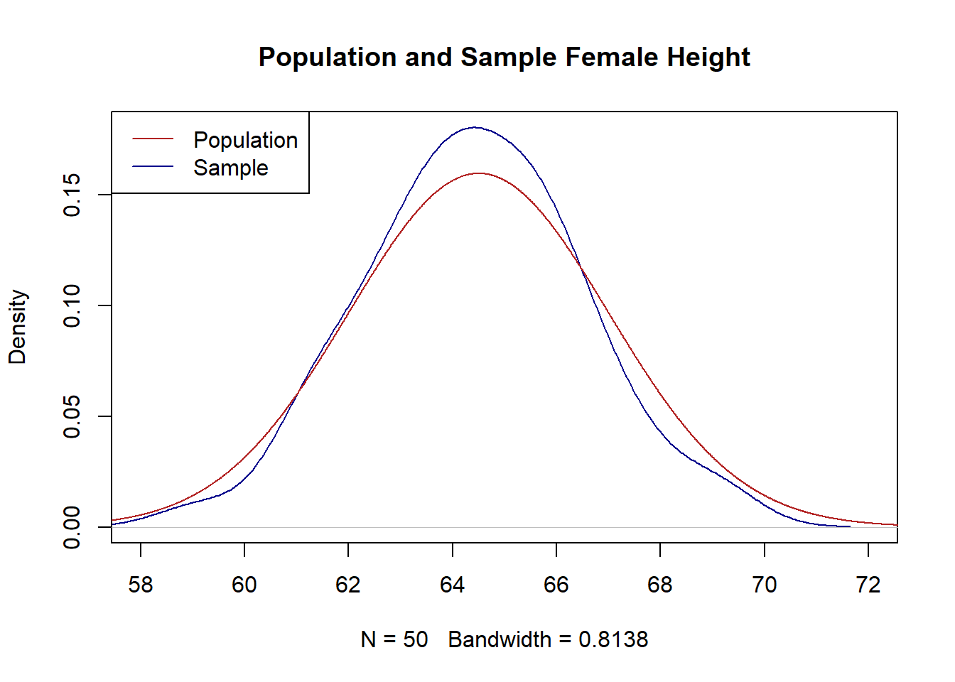

The sample is similarly shaped to the population. It is approximately normally distributed with a mean and variance that are in the ballpark of the mean and variance of the population. This is indeed what I would have expected as the sample is generated from the population, so it makes sense that they would look similar! The random seed I set ended up with a sample that is particularly close to the population, but I know with a relatively small sample size of 50 this will not always be the case.

Taking advantage of the fact that I’ve given you information about the population, plot the sampling distribution of the sample mean for \(n=50\). Confirm that this sampling distribution is correct by repeatedly sampling from this distribution, taking means, and plotting the density of those simulated means.

Via the Central Limit Theory the sampling distribution will be \(\bar{X_n}\sim N(\mu=64.5, \sigma=\frac{2.5}{\sqrt{n}})\)

#Using the population variance, the standard error is
se <- 2.5/sqrt(50)

#Draw simulated samples and mean
means <- rep(NA,10000)

for(i in 1:10000){
  means[i] <- mean(rnorm(50,64.5,2.5))
}

#Plotting the sampling distribution calculated and simulated:
eval.sd <- seq(63,66,.001)
plot(eval.sd, dnorm(eval.sd, mean=64.5, sd=se), type="l",
     main="Sampling Distribution of the Sample Mean", col="firebrick")
points(density(means), col="darkblue", type="l")
legend("topleft", c("Real Sampling Distribution", "Simulated Sampling Distribution"), lty=c(1,1), col=c("firebrick","darkblue"))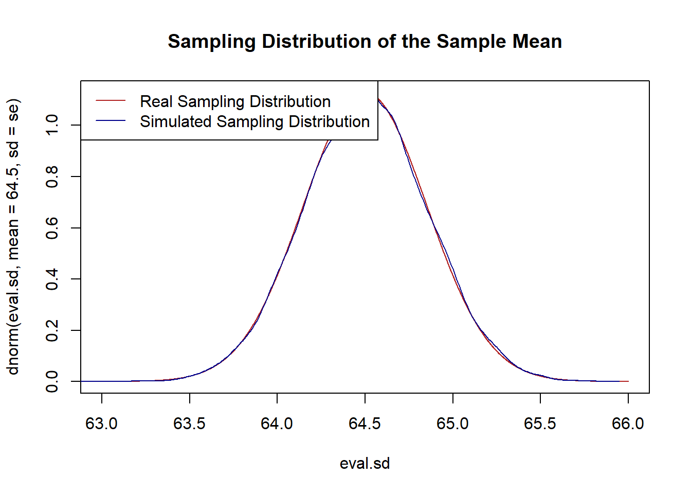

Calculate the probability that the mean height of a sample of 50 women will be less than 64 inches. Confirm your answer with the simulated results from (b).

#Calculated
pnorm(64,64.5,se)
#> [1] 0.0786496

#From simulation
mean(means<64)
#> [1] 0.0769

#Effectively the same.

Calculate the probability that the mean height of a sample of women will be between 64 and 65 inches. Confirm your answer with the simulated results from (b).

#Calculated
pnorm(65,64.5,se)-pnorm(64,64.5,se)
#> [1] 0.8427008

#From simulation
mean(means>64 & means<65)
#> [1] 0.8436

#Again, effectively the same.

What is the probability that a woman is less than 64 inches tall? What is the probability a woman is between 64 and 65 inches tall? Give the answers, and then say in words why these answers are not the same as the answers for (c) and (d).

#Prob less than 64 inches:
pnorm(64,64.5,2.5)
#> [1] 0.4207403

#Prob between 64 and 65 inches:
pnorm(65,64.5,2.5)-pnorm(64,64.5,2.5)
#> [1] 0.1585194

These are different because they are asking about the population instead of the sampling distribution. The population of women’s height is a normal distribution with expected value 64 and standard deviation of 2.5. To determine the probability of a woman having a height less than 64 inches for example, we determine the probability mass to the left of 64 in this distribution. The sampling distribution of the means of womens height is also normally distributed with a mean of 64.5, but has a standard deviation of \(2.5/\sqrt{50}\). In other words, it is a much narrower distribution. This makes sense! the range in which a bunch of means will vary is obviously smaller than how much women’s height can vary.

What size \(n\) would you need to be 99% certain that the mean height in a sample of women will be between 64 and 65 inches. Determine this answer and then repeatedly sample from the population with a sample of that size to show that 99% of sample means do indeed fall within those bounds.

We want to know the \(n\) that will make us 99% certain that samples means will be within .5 inches of the truth.

2.57 is the value of the standard normal that puts 99% of the probability mass in the center of the distribution.

We want to know what the standard error has to be such that 0.5 inches represents 2.57 standard errors:

As derived on the midterm answer key, the formula to determine the \(n\) to be 99% certain that the mean is \(\pm\) 0.5 inch of the truth is:

\[ \frac{.5}{se}=-2.57\\ \frac{.5}{\frac{sd_x}{\sqrt{n}}} = -2.57\\ .5*\frac{\sqrt{n}}{sd_x} = -2.57\\ \sqrt{n} = \frac{-2.57*sd_x}{.5}\\ n = (\frac{-2.57*2.5}{.5})^2\\ n \approx 165 \]

The math says around 165 people. Now let’s randomly sample from that distribution with that size n to determine if 99% of means are between 64 and 65:

means <- rep(NA,10000)

for(i in 1:10000){
  means[i] <- mean(rnorm(165,64.5,2.5))
}

library(dplyr)
#> Warning: package 'dplyr' was built under R version 4.1.3
#> 
#> Attaching package: 'dplyr'
#> The following objects are masked from 'package:stats':
#> 
#>     filter, lag
#> The following objects are masked from 'package:base':
#> 
#>     intersect, setdiff, setequal, union
mean(between(means, 64,65))
#> [1] 0.9906

#Yup!

Question 2

Use the code below to load the data for this question. This file contains a single sample x from an unknown distribution.

library(rio)
x <- import("https://github.com/marctrussler/IIS-Data/raw/main/Question2.RDS")

Plot the distribution of this sample and determine the mean and variance. Using your intuition: what do you expect the distribution that produced this population might have looked like? (Ignore that I tell you below, genuinely try to think about how you would answer this question if you didn’t know. )

mean(x)
#> [1] 51.75393
var(x)
#> [1] 403.601
plot(density(x))

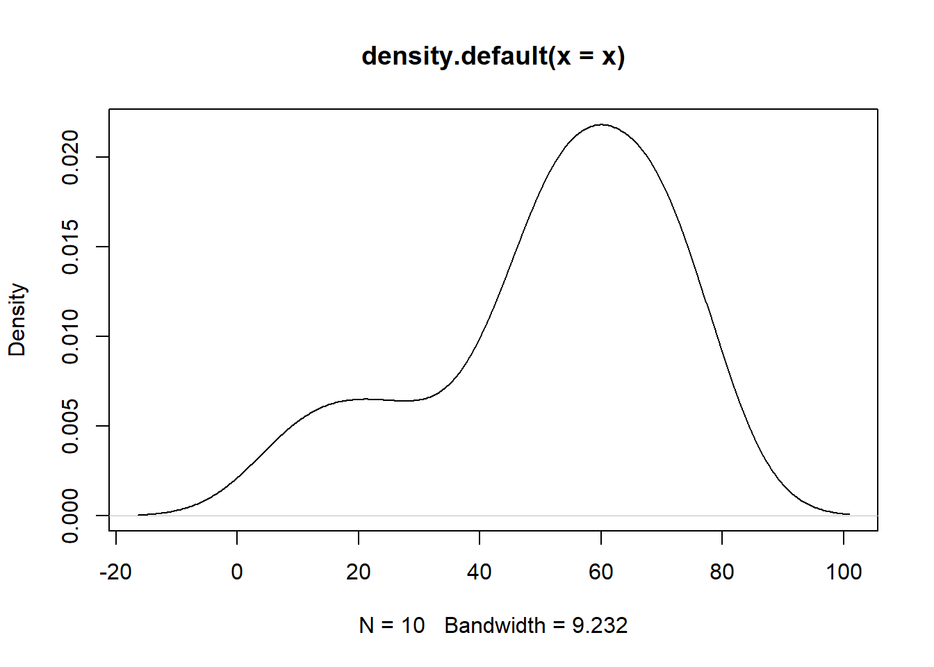
This distribution may be normal, but it also looks somewhat skewed to the left. With this few observations it’s really hard do determine what may or may not be true here. I would expect that the true mean is somehwere in the 30-70 range, but without mroe information it’s impossible to make a conclusion.

(Again ignoring that I tell you the population that this sample is drawn from below) Using only information contained in this one sample produce a 70%, 90% and 95% confidence interval around the mean of this sample. For each, describe in words what the confidence interval is telling you.

#Define the standard error
se <- sd(x)/sqrt(10)

#70%
t <- qt(.15, df=9)*-1
c(mean(x) - se*t, mean(x) + se*t)
#> [1] 44.76747 58.74038
#There is a 70\% chance the true population mean is between 44.76 and 58.74

#90%
t <- qt(.05, df=9)*-1
c(mean(x) - se*t, mean(x) + se*t)
#> [1] 40.10823 63.39962
#There is a 90\% chance the true population mean is between 40.11 and 63.4


#95%
t <- qt(.025, df=9)*-1
c(mean(x) - se*t, mean(x) + se*t)
#> [1] 37.38253 66.12532
#There is a 95\% chance the true population mean is between 37.38 and 66.12

#Can also use the language that "X% of similarly constructed confidence intervals will contain the true population mean".

The following code produced this sample: rnorm(10,56,32). Now using this information, repeatedly re-sample and calculate confidence intervals to show that 70%, 90% and 95% of similarly constructed confidence intervals contain the true population parameter.


contains.ci.70 <- rep(NA,10000)
contains.ci.90 <- rep(NA,10000)
contains.ci.95 <- rep(NA,10000)

for(i in 1:10000){
x <- rnorm(10,56,32)
se <- sd(x)/sqrt(10)

#70%
t <- qt(.15, df=9)*-1
ci <- c(mean(x) - se*t, mean(x) + se*t)
contains.ci.70[i] <- ci[1]<=56 & ci[2]>=56

#90%
t <- qt(.05, df=9)*-1
ci <- c(mean(x) - se*t, mean(x) + se*t)
contains.ci.90[i] <- ci[1]<=56 & ci[2]>=56

#95%
t <- qt(.025, df=9)*-1
ci <- c(mean(x) - se*t, mean(x) + se*t)
contains.ci.95[i] <- ci[1]<=56 & ci[2]>=56
}

mean(contains.ci.70)
#> [1] 0.6953
mean(contains.ci.90)
#> [1] 0.9007
mean(contains.ci.95)
#> [1] 0.9509

Midterm Answers

Problem Set 4