Problem Set 4

Problem Set Due Wednesday November 15th at 7pm on Canvas.

For this problem set you will hand in a .Rmd file and a knitted html output.

Please make life easy on us by using sections to clearly delineate questions and sub-questions.

Comments are not mandatory, but extra points will be given for answers that clearly explains what is happening and gives descriptions of the results of the various tests and functions.

Reminder: Put only your student number at the top of your assignment, as we will grade anonymously.

Collaboration on problem sets is permitted. Ultimately, however, the code and answers that you turn in must be your own creation. You can discuss coding strategies, code debugging, and theory with your classmates, but you should not share code or answers in any way.

Please write the names of any students you worked with at the top of each problem set.

For this problem set we are going to use the SurveyMonkey data on Pennsylvania voters from the last two weeks before the 2022 election. While this is not a perfect random sample of Pennsylvanians (or of PA voters, in particular), we can pretend like it is for the purposes of this assignment.

We are going to investigate the variable predicted.vote.prob. This is a variable that we generated which gives each individual in the data set a probability of voting from 0 to 1 based on their demographics and stated likelihood of voting.

library(rio)
sm.pa <- import("https://github.com/marctrussler/IIS-Data/raw/main/PAFinalWeeks.csv")

Without using the t.test() function, perform the 5-step hypothesis test discussed in class on the null hypothesis that predicted.vote.prob is equal to .8. (This test should be a two-tailed hypothesis test). Confirm your answer with the t.test() function.

*Specify a null and an alternative hypothesis:

\[ H_o: P(Vote)=0.8\\ H_a: P(Vote)\neq0.8 \]

Choose a test statistic and \(\alpha\)

Test statistic is the mean of predicted vote probability:

xbar <- mean(sm.pa$predicted.vote.prob,na.rm=T)

I will choose \(\alpha=.05\)

Derive the sampling distribution

I need a standard error to derive the sampling distribution, which we know the equation for:

se <- sd(sm.pa$predicted.vote.prob,na.rm=T)/sqrt(sum(table(sm.pa$predicted.vote.prob)))

To compute the p-value I must calculate a t statistic, which is the number of standard errors my test statistic is from the null.

t <- (xbar - .8)/se

I can then evaluate the total probability mass more extreme than that t statistic with \(n-1\) degrees of freedom.

pt(t, df=sum(table(sm.pa$predicted.vote.prob))-1, lower.tail=F)*2
#> [1] 3.912278e-16

(While you will get the same result from using the normal distribution, for full points you must use the \(t\) distribution.)

Reject the null hypothesis if \(p\) is less than \(\alpha\).

The probability of seeing a result this extreme if the true average predicted probability of voting was .8 is very small, less than 1%. As such I reject the null hypothesis that the true average predicted probability of voting is 80%.

The results are the same using the t.test function.

t.test(sm.pa$predicted.vote.prob, mu=.8)
#> 
#>  One Sample t-test
#> 
#> data:  sm.pa$predicted.vote.prob
#> t = 8.1684, df = 5060, p-value = 3.912e-16
#> alternative hypothesis: true mean is not equal to 0.8
#> 95 percent confidence interval:
#>  0.8228702 0.8373148
#> sample estimates:
#> mean of x 
#> 0.8300925

Again, without using the t.test() function, perform the 5-step hypothesis test discussed in class on the null hypothesis that those who identify as Democrats and Republicans have equal predicted probabilities of voting. (So you don’t have to calculate it with a terrible equation, the degrees of freedom for the t-test will be 3543.9.) Confirm your calculated answer using the t.test() function.

Generate a variable indicating if someone is a D or R

sm.pa$d.vs.r <- NA
sm.pa$d.vs.r[sm.pa$pid=="Democrat"]<- 1
sm.pa$d.vs.r[sm.pa$pid=="Republican"]<- 0

Specify a null and an alternative hypothesis:

\[ H_o: P(Vote|Dem) - P(Vote|Rep)=0\\ H_o: P(Vote|Dem) - P(Vote|Rep) \neq 0\\ \]

Choose a test statistic and \(\alpha\)

Test statistic is the difference in means

diff.means <- mean(sm.pa$predicted.vote.prob[sm.pa$d.vs.r==1],na.rm=T) - 
                     mean(sm.pa$predicted.vote.prob[sm.pa$d.vs.r==0],na.rm=T)

I will choose \(\alpha=.05\)

Derive the sampling distribution

I need a standard error to derive the sampling distribution, which we know the equation for:

se <- sqrt((var(sm.pa$predicted.vote.prob[sm.pa$d.vs.r==1], na.rm=T)/sum(sm.pa$d.vs.r==1,na.rm=T)) +
           (var(sm.pa$predicted.vote.prob[sm.pa$d.vs.r==0], na.rm=T)/sum(sm.pa$d.vs.r==0,na.rm=T))   )

To compute the p-value I must calculate a t statistic, which is the number of standard errors my test statistic is from the null.

t <- (diff.means - 0)/se

I can then evaluate the total probability mass more extreme than that t statistic with the stated degrees of freedom.

pt(t, df=3543.9, lower.tail=F)*2
#> [1] 1.265051e-05

(Again, while you will get the same result from using the normal distribution, for full points you must use the \(t\) distribution.)

Reject the null hypothesis if \(p\) is less than \(\alpha\).

The probability of seeing a result this extreme if the true difference in means was 0 is very small, less than 1%. As such I reject the null hypothesis that Democrats and Republicans have an equal probability of voting.

And again, we get the same result from the t.test function:

t.test(sm.pa$predicted.vote.prob ~ sm.pa$d.vs.r)
#> 
#>  Welch Two Sample t-test
#> 
#> data:  sm.pa$predicted.vote.prob by sm.pa$d.vs.r
#> t = -4.3723, df = 3543.9, p-value = 1.265e-05
#> alternative hypothesis: true difference in means between group 0 and group 1 is not equal to 0
#> 95 percent confidence interval:
#>  -0.04656905 -0.01773390
#> sample estimates:
#> mean in group 0 mean in group 1 
#>       0.8610535       0.8932050

Assume that the difference in the predicted probability of turning out in Democrats vs. Republicans (about 3.2%) is the truth in the population. Using the methodology from class, visualize and calculate \(\beta\), the probability of a false negative, for the hypothesis test from (2). Similar to what I did in class, you can assume (for this question, not above) that the sampling distribution of the difference in means is normally distributed, as opposed to \(t\) distributed. Describe briefly what you see in your visualization and how it relates to your calculated \(\beta\).

Using the standard error calculated above, plot the true sampling distribution (centered on 3.2%) and the null sampling distribution (centered on 0). I will also plot the zone in which we will fail to reject the null hypothesis for an \(\alpha\) of .05, which ranges \(\pm 1.96*se\) above and below the null hypothesis.

eval <- seq(-.03,.06,.0001)
plot(eval,dnorm(eval, mean=0, sd=se), type="l", col="darkblue")
points(eval,dnorm(eval, mean=.032, sd=se), type="l", col="firebrick")
abline(v=c(1.96*se, -1.96*se), col="darkblue", lty=2)
legend("topleft", c("Null Sampling Distribution", "True Sampling Distribution"))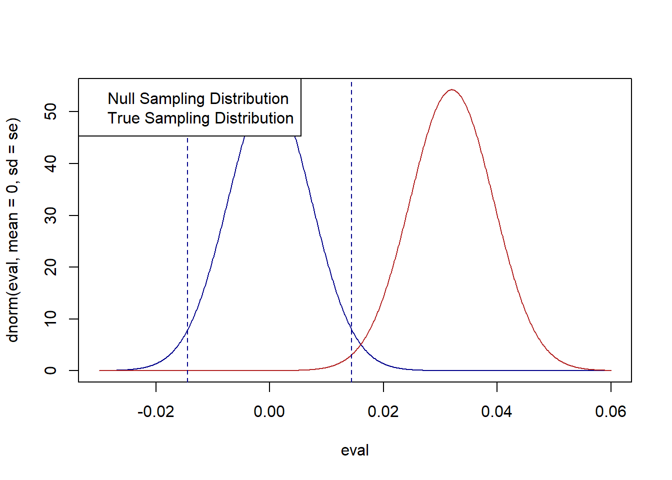


#Calculate area under red curve that is in-between the two blue lines
pnorm(1.96*se, mean=.032, sd=se)-pnorm(-1.96*se, mean=.032, sd=se)
#> [1] 0.008386349

The probability of a false negative in this hypothesis test is very small, only around .8%. We can see this visually in the plot above. The red distribution is the true sampling distribution that is generating means. The blue distribution is what we assume under the null hypothesis. The area in between the two lines is the zone where, if a sample mean is drawn there, we will falsely fail to reject the null hypothesis. Very few “true” means will be generated in that area, which is signified by a very small overlap between the red distribution and that zone.

Having seen the results of (3), I might be concerned that I have wasted my money getting so many respondents. Calculate and visualize \(\beta\) for sample sizes ranging from 100 to 10000. Eye-balling it, what sample size would result in a \(\beta\) of 20%? You can again assume that the difference of means in the sample is representative of the true population difference in means. You can further assume that the sample variances for each of the groups is representative of the true variances in the population. Finally, for simplicity assume that each sample is 50/50 Democrats and Republicans.

#For each sample size need a standard error
var.dem <- var(sm.pa$predicted.vote.prob[sm.pa$d.vs.r==1], na.rm=T)
var.rep <- var(sm.pa$predicted.vote.prob[sm.pa$d.vs.r==0], na.rm=T)

n <- seq(100,10000,1)
se <- sqrt((var.dem/(n/2))+
           (var.rep/(n/2)))
beta <- pnorm(1.96*se, mean=.032, sd=se)-pnorm(-1.96*se, mean=.032, sd=se)

plot(n, beta, type="l", main="False Negative Rate")
abline(h=.2, lty=2)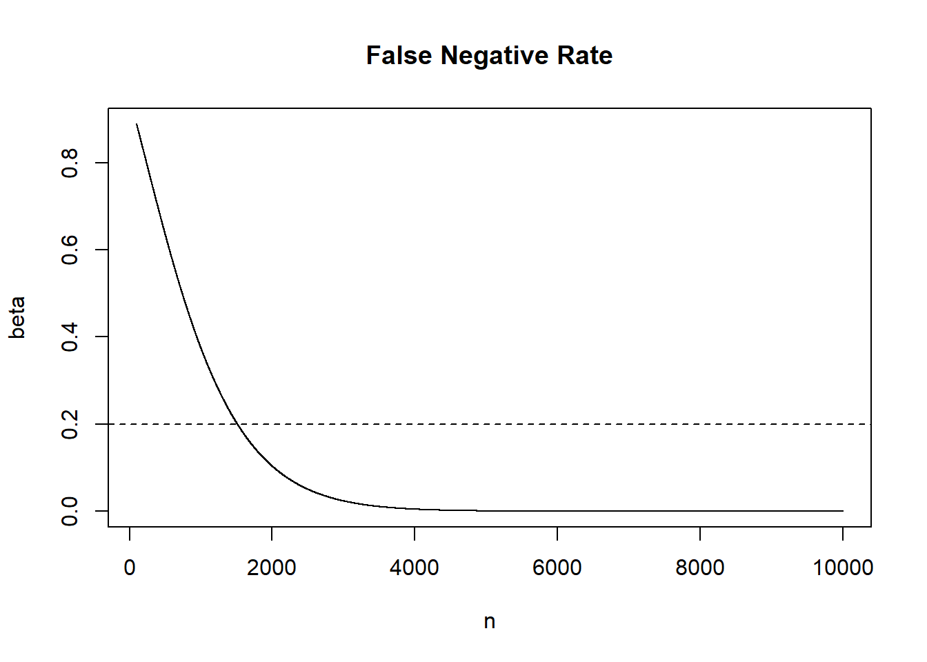

We now want to investigate the relationship between age and predicted.vote.prob. Create a scatterplot with age on the x-axis and predicted.vote.prob on the y-axis. Briefly describe what you see.

plot(sm.pa$age, sm.pa$predicted.vote.prob)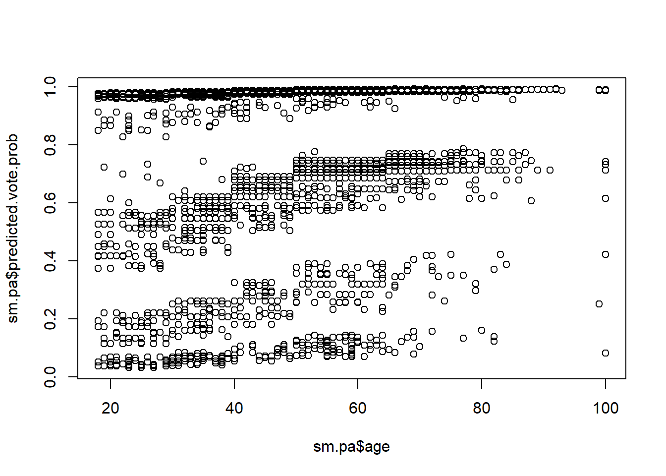

Without using the cov() and cor() functions, calculate the covariance and correlation of age and predicted.vote.prob. Confirm your answers using the cov() and cor() functions. In political terms, what do these numbers mean?

#Covariance
cov <- (1/5060)*sum( (sm.pa$age - mean(sm.pa$age)) *(sm.pa$predicted.vote.prob - mean(sm.pa$predicted.vote.prob))  )
cov
#> [1] 1.463317
cov(sm.pa$age, sm.pa$predicted.vote.prob)
#> [1] 1.463317

#Correlation
cor <- cov/sqrt( var(sm.pa$age)*var(sm.pa$predicted.vote.prob) )
cor
#> [1] 0.3531501
cor(sm.pa$age, sm.pa$predicted.vote.prob)
#> [1] 0.3531501

There is a mildly positive relationship between age and the predicted probability of voting. Politically, this means that older people were deemed to be slightly more likely to turn out to vote in the upcoming election than were younger people.

Is the correlation you found in (6) statistically distinguishable from 0? Use the bootstrap to generate a sampling distribution around this correlation, and determine the 95% confidence interval using the quantile() function.

#Generate 10000 bootstrap samples and calculate correlation in each

bs.cors <- rep(NA,10000)

for(i in 1:length(bs.cors)){
bs.data <- sm.pa[sample(1:nrow(sm.pa), nrow(sm.pa), replace=T),]
bs.cors[i] <- cor(bs.data$age, bs.data$predicted.vote.prob)
}

quantile(bs.cors,.025)
#>      2.5% 
#> 0.3262874
quantile(bs.cors,.975)
#>     97.5% 
#> 0.3792464

The bootstrap 95% CI ranges from .32 to .37. In other words, there is around a 95% chance that the true population correlation coefficient is within those bounds. Becuase these bounds are so far from 0, I am confident in rejecting the null hypothesis that the true correlation in the population is 0.

Problem Set 3

Problem Set 5