Problem Set 2

Problem Set Due Wednesday October 11 at 7pm on Canvas.

For this problem set you will hand in a .Rmd file and a knitted html output.

Please make life easy on us by using sections to clearly delineate questions and sub-questions.

Comments are not mandatory, but extra points will be given for answers that clearly explains what is happening and gives descriptions of the results of the various tests and functions.

Reminder: Put only your student number at the top of your assignment, as we will grade anonymously.

Collaboration on problem sets is permitted. Ultimately, however, the code and answers that you turn in must be your own creation. You can discuss coding strategies, code debugging, and theory with your classmates, but you should not share code or answers in any way.

Please write the names of any students you worked with at the top of each problem set.

Question 1

Solve the following questions about the specified Binomial (\(B\)), Uniform (\(U\)) and Normal (\(N\)) random variables:

\(Y \sim B(n=500, \pi=.45)\)

\(E[Y]\)

500*.45
#> [1] 225

\(V[Y]\)

500*.45*(1-.45)
#> [1] 123.75

\(P(Y=150)=\)?

dbinom(150, 500, .45 )
#> [1] 2.220032e-12

\(P(Y \leq 200)=\)?

pbinom(200, 500, .45)
#> [1] 0.01356437

\(P(200<Y<223)=\)?

pbinom(222, 500, .45) - pbinom(200, 500, .45) 
#> [1] 0.3980971

We want to add up the probability of 201,201,203….222. We do not want to include the probability of 223 (so we start with all the probability up to including 222) and we do not want to include the probaility of 200 (so we make sure to subtract off all the probability to the left of, and including, 200).

Visually:

out.nums <- c(195:200,223:227)
out.probs <- pbinom(out.nums, size=500, prob=.45)
in.nums <- 201:222
in.probs <- pbinom(in.nums, size=500, prob=.45)  
plot(out.nums, out.probs, col="firebrick", pch=16, ylim=c(-.1, .7))
points(in.nums, in.probs, col="forestgreen", pch=16)
segments(190,-.05, 200, -.05)
segments(190,-.1, 222, -.1)

\(P(200\leq Y \leq 223)=\)?

pbinom(223, 500, .45) - pbinom(199, 500, .45) 
#> [1] 0.436247

We want to add up the probability of 200,201,201,203….223. We now want to include the exact probability of 223 (so we start with all the probability up to including 223) and we do want to include the probability of 200 (so we make sure not to subtract off it’s probability so we subtract off all the probability to the left of, and including, 199).

Visually:

out.nums <- c(195:199,224:227)
out.probs <- pbinom(out.nums, size=500, prob=.45)
in.nums <- 200:223
in.probs <- pbinom(in.nums, size=500, prob=.45)  
plot(out.nums, out.probs, col="firebrick", pch=16, ylim=c(-.1, .7))
points(in.nums, in.probs, col="forestgreen", pch=16)
segments(190,-.05, 199, -.05)
segments(190,-.1, 223, -.1)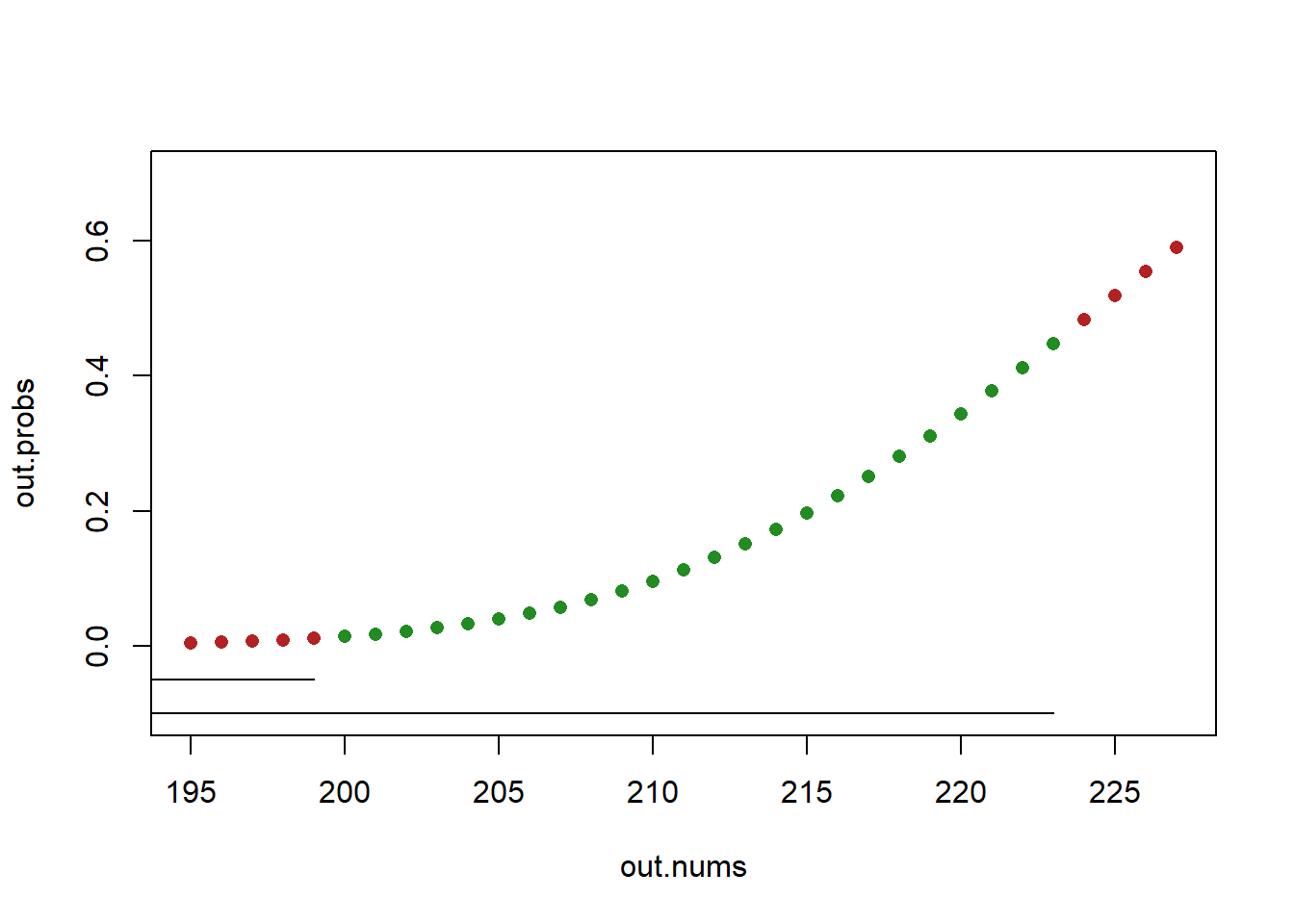

\(Q \sim U(min=10, max=200)\)

\(E[Q]\)

(10+200)/2
#> [1] 105

\(V[Q]\)

((200-10)^2)/12
#> [1] 3008.333

\(P(Q=12)=\)?

dunif(12, min=10, max=200)
#> [1] 0.005263158

This gives an answer because it is the graphing value of the PDF at this value, but the correct answer is 0, because the probability of any specific value of a continuous RV is 0.

\(P(12<Q<20)=\)?

punif(20, 10,200) - punif(12, 10,200)
#> [1] 0.04210526

\(P(12\leq Q \leq20)=\)?

Trick question! Same answer. Because the probability of being exactly equal is zero this doesn’t change the way we calculate this at all.

punif(20, 10,200) - punif(12, 10,200)
#> [1] 0.04210526

\(X \sim N(\mu=26, \sigma^2=49)\)

\(p(X>30) =\) ?

pnorm(30,26,7, lower.tail=F)
#> [1] 0.2838546

\(p(24 < X < 30) =\) ?

pnorm(30, 26, 7) - pnorm(24, 26, 7)
#> [1] 0.3285969

Solve for \(i\) where \(p(X<i)=.75\)

qnorm(.75, 26,7)
#> [1] 30.72143

Solve for \(i,j\) where \(p(i<X<j)=.85\)

.925-.075
#> [1] 0.85
qnorm(.075, 26,7)
#> [1] 15.92328
qnorm(.925, 26,7)
#> [1] 36.07672

Solve for \(c\) such that \(p(X < 45) = p(Z < c)\), where \(Z \sim N(0, 1)\)

#What probability is less than 45 in this normal distribution?
pnorm(45, 26,7)
#> [1] 0.9966791

#For the standard normal, what puts that amount of probability in the left tail?
qnorm(pnorm(45, 26,7))
#> [1] 2.714286

Question 2

Women’s height is normally distributed with mean of 64 and a standard deviation of 3. Using this linked table, and without using R (you can use it as a calculator but can’t use the norm functions): what is the approximate probability a woman has a height between 63 and 66 inches? In a few sentence describe how you got your answer.

How many SD’s above and below the mean are those two points?

(63-64)/3
#> [1] -0.3333333
(66-64)/3
#> [1] 0.6666667

After finding these two points I can use the attached Z-table to look up the probability to the left of those two points in the standard normal distribution. Using the table I find that to the left of -.33 (which is .33 standard deviations below the mean for any normal distribution) is a probability mass of .37. Similarly, using the table I find that to the left of .67 (which is .67 standard deviations above the mean for any normal distribution) is .75 probability mass. As such the probability between these two points is: \(.75-.37=.38=38\%\). 38% of the probability mass is between .33 standard deviations below the mean and .67 standard deviations above the mean. Put back into the terms of the original question: approximately 38% of women are between 63 and 66 inches tall. (Your answer will be around here depending on rounding.)

Question 3

Consider the following probability mass function of a random variable, \(K\):

\[ f(K) = p(K=k) = \begin{cases} \frac{1}{6} \text{ if } 1\\ \frac{1}{3} \text{ if } 2\\ \frac{1}{3} \text{ if } 4\\ \frac{1}{6} \text{ if } 10\\ \end{cases} \]

What is the CDF of \(k\)?

The CDF of K is:

\[ F(K) = p(K < k) = \begin{cases} 0 \text{ if } K <1\\ \frac{1}{6} \text{ if } 1\leq k <2\\ \frac{1}{2} \text{ if } 2\leq k <4\\ \frac{5}{6} \text{ if } 4\leq k <10\\ 1 \text{ if } 10\leq k\\ \end{cases} \]

What is the expected value of K?

The expected value of K is:

\[ \begin{align} E[K] = &\sum k*f(k)\\ = &1*\frac{1}{6} + 2*\frac{1}{3} + 4*\frac{1}{3} + 10*\frac{1}{6}\\ = & 3.833\\ \end{align} \]

What is the variance of K?

\[ \begin{align} E[X^2]= &1^2*\frac{1}{6} + 2^2*\frac{1}{3} + 4^2*\frac{1}{3} + 10*^2\frac{1}{6}\\ = &23.5\\ E[X]^2 = &3.83^2 = 14.6689\\ V[K] = &E[X^2] - E[X]^2\\ = &23.5-14.6689\\ = & 8.83 \end{align} \]

Use R to draw 10,000 samples of K. Confirm that the expected value and variance you calculated above is roughly correct.

set.seed(19104)
#Option 1:
coin <- c(rep(1,10), rep(2,20), rep(4,20), rep(10,10))
samp <- sample(coin, 10000, replace=T)

#Option 2 (slightly cleaner)
samp <- sample(c(1,2,4,10),10000, prob=c((1/6), (1/3), (1/3), (1/6)), replace = T)

mean(samp)
#> [1] 3.864
var(samp)
#> [1] 8.992203

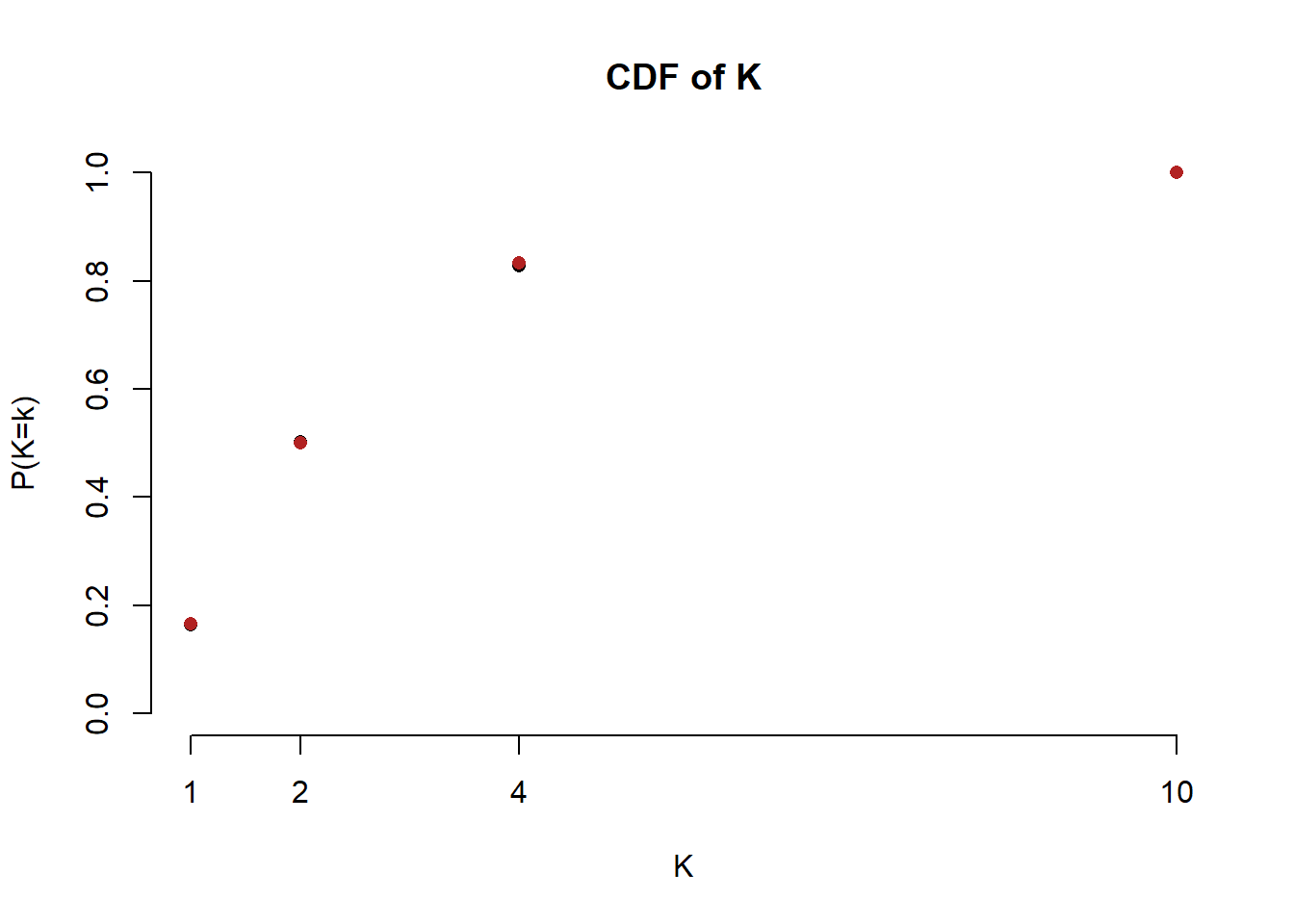
#Both Match

Plot the PMF and CDF of K, comparing the simulated and calculated values. For the CDF try out the cumsum() function.

#PMF
values <- sort(unique(samp))
probs <- prop.table(table(samp))
true.probs <- c((1/6), (1/3), (1/3), (1/6))
plot(values, probs, pch=16, ylim=c(0,.4), axes=F,
     xlab="K", ylab="P(K=k)",
     main="PMF of K", col="darkblue")
axis(side=2)
axis(side=1, at=c(1,2,4,10))
points(values, true.probs, col="firebrick", pch=16)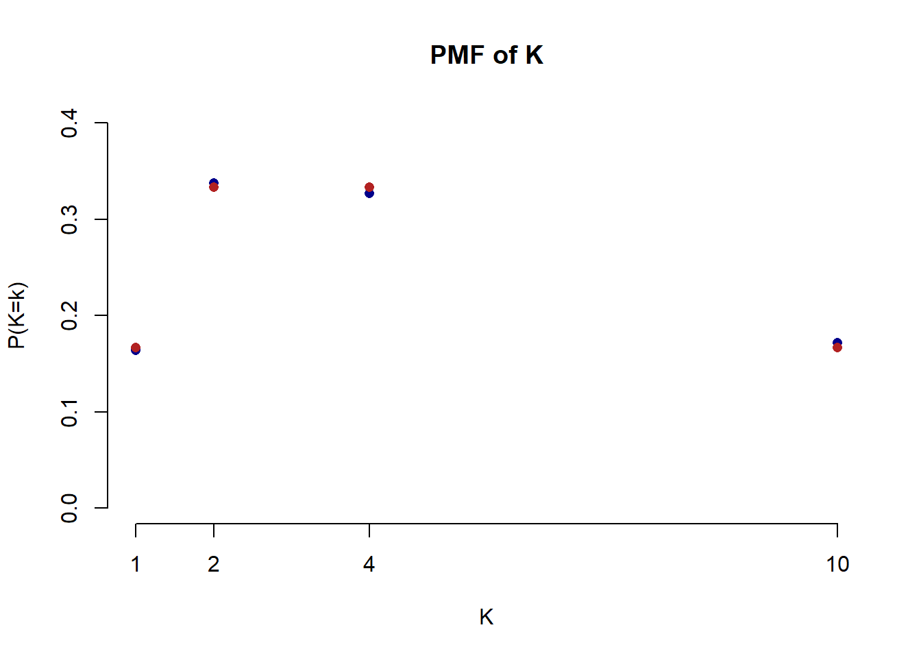


#CDF

probs.cdf <- cumsum(probs)
true.probs.cdf <- cumsum(true.probs)

plot(values,cumsum(probs), pch=16, ylim=c(0,1), axes=F,
     xlab="K", ylab="P(K=k)",
     main="CDF of K")
axis(side=2)
axis(side=1, at=c(1,2,4,10))
points(values, true.probs.cdf, col="firebrick", pch=16)

Problem Set 1

Midterm Answers