Midterm Answers
Question 1 (15 points)
(a) Back home in Canada the main lottery is “Lotto 6/49”. In this lottery you select 6 numbers from 1 to 49. For the drawing, 49 numbered balls are placed in a bin and 6 are randomly selected. You win the grand prize if the 6 balls drawn are the same as the 6 numbers you selected. What are the odds of winning this lottery? What would the odds of the lottery be if you had to select 6 numbers AND the balls had to be drawn in the same order as the 6 numbers you selected? Why is this second number higher/lower?
The lottery is a combination because order doesn’t matter. You have one set up numbers and there are \(_{49}C_{6}\) possible sequences of numbers. So the odds of winning the lottery are 1 in:
choose(49,6)
#> [1] 13983816
If you also had to match the order of numbers this would be a permuatation, which is given by \(_{49}P_{6}\). If this was the case the odds of winning the lottery are 1 in:
A way bigger number!
The second number is bigger because every unique sequence of numbers is counted. There are \(6!\) ways to organize each combination of 6 numbers, so the number of possibilities is that much larger.
(b) Sticking with the above 6/49 lottery. What if a shady Canadian government employee approached you and offered to tell you one, two, three, four, or five of the six numbers that will be drawn in the next drawing. If the grand prize is 30 million dollars and the lottery costs $2, how much should you be willing to pay to learn, one, two, three, four, or five numbers? Assume that the only prize is the grand prize. Hint: think of this as a random variable where you either lose 2 dollars with some probability, or win 29,999,998 (the prize minus the cost) dollars with some probability.
We can think about the lottery as a random variable where you lose 2 dollars if you don’t match all the numbers, and you get 2,999,998 dollars if you match all the numbers. So the raw expected value is:
If I know 1 of the numebrs however, I now only have to pick 5 numbers correctly out of 48 to win 30 million dollars:
Note that both the numbers I have to match (5) and the numbers I have to choose from (48) change from the original ocassion. I no longer am choosing from 49 numbers!
The difference between these two expected values is what I should pay.
Now filling this in for all of them:
(c) Every Thursday night my wife and I play 3 games of cribbage (because we are very old). Let’s say that If you looked at all the cribbage games we have ever played my wife has won 65% of them. Given that true skill level, what is the probability that I win zero, one, two, or three games on a Thursday night? Calculate these 4 quantities mathematically without using built in R functions. That is, you can use algrebra and R as a calculator, but cannot use any of the built in distribution functions.
We can answer this question with the binomial formula:
\[ P(K=k) = _nC_k * P(k)^k *P(1-k)^{n-k}\\ \]
Putting this into R:
k <- c(0,1,2,3)

p <- choose(3,k)*(.35^k)*(.65^{3-k})

cbind(k,p)
#>      k        p
#> [1,] 0 0.274625
#> [2,] 1 0.443625
#> [3,] 2 0.238875
#> [4,] 3 0.042875
If my wife’s chance of winning any given game is 65% then my chance is 35%. Plugging that into the binomial formula I have a 27% chance of winning no games, a 44% chance of winning 1 game, a 23% chance of winning 2 games, and a 4.2% chance of winning all 3 games.
Question 2 (35 points)
On December 1, 1969 a lottery was held to determine which American men would be drafted to fight in the Vietnam War. All birthdays (including leap day, February 29th) were placed in a large bin and selected one at a time and the order was recorded. The first birthday drawn was September 1st, so men born on September 1st between 1944 and 1950 were the fist drafted. The second birthday drawn was April 24th, so men born on that day between 1944 and 1950 were the second group drafted. Ultimately, men from the first 195 numbers drawn were drafted for the war.
(a) Consider a random variable representing the probability that you are born in each month of the year, where January is month 1, February is month 2 etc.: \(P(BornMonth=Month_i)\). What is the PMF of this random variable? (Remember that not all months have the same number of days). For the sake of simplicity (and to match the draft data), assume that February always has 29 days and there are always 366 days in the year. Use R to graph this PMF, where the x-axis should be months 1 through 12, and the y-axis the probability of being born in that month.
To determine this I make a vector of the number of days in each month and divide each quantity by 366 (the number of days in a leap year).
days.of.the.month <- c(31,29,31,30,31,30,31,31,30,31,30,31)
prob.month <- days.of.the.month/366

plot(1:12,prob.month, col="darkblue", pch=16, main="P(Born in Month)",
     xlab="Month", ylab="Probability",ylim=c(.05,.15))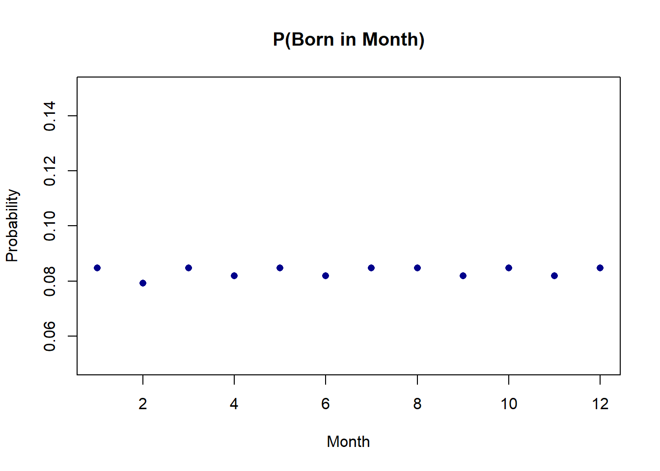
(b) Mathematically calculate the expected value and variance of this random variable.
The expected value of a random variable is \(E[X]=\sum xP(x)\). As such, I multiply the number of the month by the probability of that month occurring. The variance is given by \(V[X]=E[X^2] - E[X]^2\). As such I find the expected value of the random variable squared, and subtract off the square of the random variable.
#Expected Value
exp <- sum((1:12)*prob.month)
exp
#> [1] 6.513661
#Variance
var <- sum(((1:12)^2) *prob.month) - exp^2
var
#> [1] 11.91102
(c) The file “VietnamDraft.Rds” contains the actual results of the 1969 draft. You can load the data by copying and pasting the code below into your Rmarkdown.
library(rio)
vietnam.draft <- import("https://github.com/marctrussler/IIS-Data/raw/main/VietnamDraft.Rds")
In the data day.of.year gives the days of the year sequentially numbered from 1 (January 1st) to 366 (December 31). month and day give the corresponding month and day for that day of the year. draft.number is the selected draft number for that date, where day 1 is the first group selected, day 2 the second, etc. Remembering that the first 195 draft numbers were called, determine the probability of being born in each month, conditional on being selected for the draft \(P(BornMonth=Month_i| DraftNumber<=195)=?\). Plot these values alongside the unconditional probability of being born in each month you calculated above. Just looking visually: would you conclude that the RV which describes the probability you are born in each month generated the draft selection data? What does this mean in real terms?
I want to determine the probability of being born each month conditional on being drafted. Using the conditional probability formula this means that:
\[ P(BornMonth=Month_i| DraftNumber<=195)=\frac{P(BornMonth=Month_i \& DraftNumber<=195)}{P(DraftNumber<=195)} \] To get this conditional probability I have to determine the probability in each month for both of these things being true, and divide it by the probability of being drafted overall. So for January (for example), I need to find the probability of being born in January AND being drafted, and divide that by the probability of being drafted. I use a loop to go through each month sequentially calculating this value, and then plot that value beside the unconditional probability.
months <- unique(vietnam.draft$month)
prob.selected <- rep(NA, length(months))
for(i in 1:length(months)){
  prob.selected[i] <- mean(vietnam.draft$month==months[i] & vietnam.draft$draft.number<=195)/mean(vietnam.draft$draft.number<=195)
}

plot(1:12,prob.month, col="darkblue", pch=16, ylim=c(.05,.15), xlab="Month",
     ylab="Probability", main="Comparison of PMFs")
points(1:12, prob.selected,col="firebrick", pch=16)
legend("topleft", c("P(Born in Month)", "P(Born in Month | Selected for Draft)"), pch=c(16,16),
       col=c("darkblue", "firebrick"))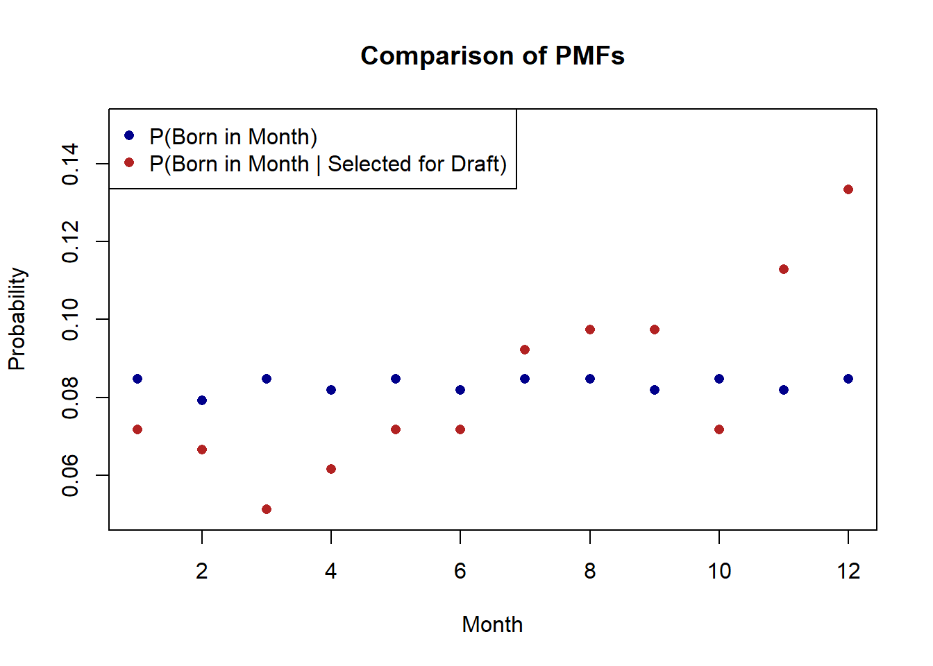
(There are a couple of other ways to do this, but above is what I thought to do.)
The red dots look very different from the blue dots. The probability of being born in a month early in the year conditional on being drafted is much lower than the unconditional probability of being born in one of those months. On the other hand, the probability of being born late in the year conditional on being drafted is much higher than the unconditional probability of being born in these months. It seems unlikely (although not definitive) that the blue random variable could create the red dots.
In real terms it seems like the 1969 Vietnam Draft did not select random birth dates successfully. While not every draftee ultimately served in Vietnam, this error had tragic consequences for those selected, particular if you consider that draftees were more likely to die in the war. You can read more about what happened here (if you haven’t already). The draft procedure was changed substantially in subsequent years and led to a more random selection.
(d) December should be the month with one of the largest difference between \(P(BornMonth=Month_i)\) and \(P(BornMonth=Month_i|Selected)\). Design a simulation in R to visually show that this large difference for December likely didn’t occur simply by random chance. Hints: You don’t need to worry about the exact days drafted. Instead think about each “draft” being 195 birth months. Think about how you can use the provided data set to do your sampling. Do you want to sample with or without replacement? My method of determining the relative likelihood is to plot the density of my simulated \(P(BornDecember|Selected)\) and showing where the actual value of \(P(BornDecember|Selected)\) is, but you can choose whatever comparison makes sense to you.
We don’t care which particular day a draftee was born in, only the month. So each of the 195 selections will be a month of the year. If the draft was “fair” the 195 drafted birth-months would be drawn in exact proportion to the probability of being born in that month. As such, I sample from the month column of the included dataset (which has all the dates) 195 times. I sample without replacement because a date cannot be selected twice. There should be around 8.5% of the draft days in December, because that’s the actual rate of birthdays in December. To get the probability of being born in that month conditional on being drafted, I divide the number of draft days that are December by the number of total draft days (195).
To determine whether the observed value was particular, or not, I plot a density of all of the simulated drafts that are based on the probability of being born in December and compare the observed value of .13. This value definitely stands out, which further solidifies the idea that the draft was unfair.
prob.december <- rep(NA, 1000)
for(i in 1:1000){
  samp.month <- sample(vietnam.draft$month,195, replace=F)
  prob.december[i] <- sum(samp.month==12)/195
}

plot(density(prob.december), main="Simulated P(December|Selected)", xlab="Probability")
abline(v=prob.selected[12], lty=2, col="firebrick")
legend("topleft", "True P(December|Selected", lty=2, col="firebrick")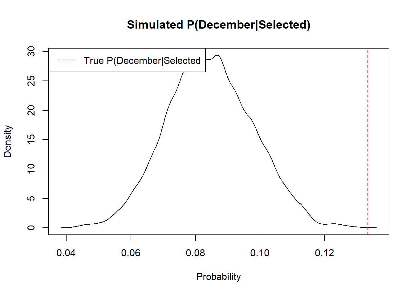
Question 3 (20 points)
Consider the following estimator for the expected value of a population (i.e. a replacement for the mean):
\[ \phi = \frac{X_1 + X_2 + X_3}{3} \]
The estimator, \(\phi\) (phi), simply takes the average of the first three observations of any dataset, regardless of the length of that dataset.
(a) What is the expected value of \(\phi\)? Is this estimator unbiased?
To be unbiased the expected value of the estimator must equal \(E[X]\) because unbiasedness is \(E[X] - E[\phi]=0\)?
\[ E[\phi] = E[\frac{X_1 + X_2 + X_3}{3}]\\ = \frac{1}{3}*E[X_1 + X_2 + X_3]\\ = \frac{1}{3}*E[X_1] + E[X_2] + E[X_3]\\ =\frac{1}{3}*E[X] + E[X] + E[X]\\ =\frac{1}{3}*3*E[X]\\ =E[X] \]
This estimator is unbiased.
(b) What is the variance of \(\phi\)? Is this estimator consistent? What would a graph of the Mean Squared Error (MSE) of this graph look like from sample size 10 to 1000 (just describe it in words)?
We can similarly take the variance of this estimator:
\[ V[\phi] = V[\frac{X_1 + X_2 + X_3}{3}]\\ = \frac{1}{9}V[X_1 + X_2 + X_3]\\ =\frac{1}{9}*V[X] + V[X] + V[X]\\ = \frac{1}{9}*3*V[X]\\ =\frac{V[X]}{3} \]
No this is not a consistent estimator. A consistent estimator has a variance that gets smaller as the \(n\) increases, and here the variance will stay the same regardless of the sample size.
MSE is \(Variance +Bias^2\). Here because bias is 0 the MSE would be a flat horizontal line that would be equal to the variance of the underlying variable divided by 3.
(c) Use simulation to apply this estimator to a random variable of your choosing a large number of times. (This should work for any distribution you want to sample from!) Use your simulation to show that this estimator is unbiased and has a variance equal to what you calculated above.
phi.estimate <- rep(NA, 10000)
for(i in 1:length(phi.estimate)){
phi.estimate[i] <- sum(rnorm(100, mean=3, sd=3)[1:3])/3
}

#Is sampling distribution centered on the true population expected value of 3?

plot(density(phi.estimate), xlab="Phi",
     ylab="Density", main="Sampling distirbution of Phi")
abline(v=3, lty=2, col="firebrick")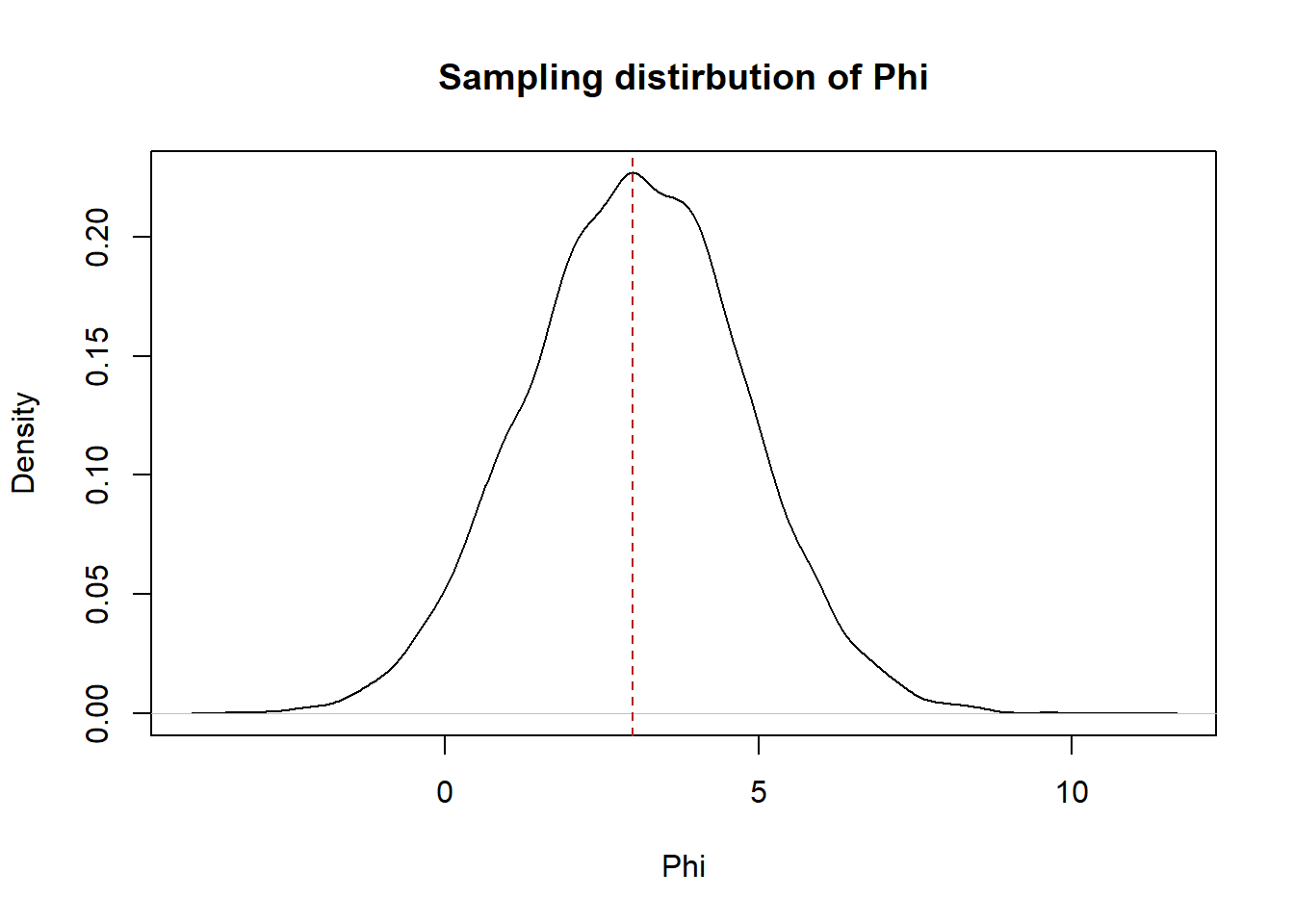
It is centered on the population expected value.
We expect that the variance will be \(\frac{V[x]}{3} = \frac{9}{3}=3\).
var(phi.estimate)
#> [1] 3.004747
It is!
Question 4 (30 points)
“ElectionData1801Midterm.RData” contains results from the 2020 presidential election. You can load the data by copying and pasting the R code below into your Rmarkdown. For each state plus DC I have given the two party percentage won by Biden (i.e. the percentage of the vote won by Biden among those who voted for Biden or Trump). Consider this the true level of support for Biden in each of these states.
library(rio)
elect <- import("https://github.com/marctrussler/IIS-Data/raw/main/ElectionData1801Midterm.Rds")
Consider performing a poll of 500 people in each of these states. In each poll an estimate of the proportion of voters who support Biden would be calculated (i.e. the mean of the variable telling us whether each person supports Biden over Trump).
We know that each time we take a sample of 500 people and calculate a mean/proportion we will get a slightly different answer. Answer the following questions about the variability/distribution in these estimates of Biden’s support:
The purpose of this question is to recognize that each sample mean is drawn from a normal distribution with parameters that are determined by the particular Bernoulli we are sampling from in each state and the sample size of 500. It is possible to get approximately the right answer using the binomial distribution, though that’s not what the question prompts you to do, given that I explicitly talked about the distribution of sample means/proportions. Additionally, I do not believe it is possible to answer the bonus question without using the standard normal distribution.
(a) Add a new column to the data set which gives, for each state, the probability that the proportion of Biden’s support from a poll of 500 people will be within 2 percentage points of the true value in that state. For example if the true support for Biden in a state is 52.5%, what is the probability a poll of 500 people will have an estimate of Biden support that is between 50.5% and 54.5%?
We are drawing from a Bernoulli Random Variable (the probability of Biden winning in each state) and forming means.
Using our knowledge of sampling and the Central Limit Theorem, the sample means in each of these states will be: \(N(\mu=Biden.Perc_i, \sigma^2=\frac{Biden.Perc_i*(1-Biden.Perc_i)}{500}\)
First calculate the standard error of the sampling distribution in each state, which is the square root of the variance of the Bernoulli random variable divided by the sample size:
elect$se <- sqrt((elect$biden.perc*(1-elect$biden.perc))/500)To get the proportion of means that will be within 2 percentage points of the truth for each states, for each of the sampling distributions I can subtract the probability that is to the left of \(\mu-.02\) from the probability that is to the left of \(\mu+.02\), leaving just the probability that is in the middle.
elect$prop.within.2 <- pnorm(elect$biden.perc+.02, mean=elect$biden.perc, sd=elect$se) - pnorm(elect$biden.perc-.02, mean=elect$biden.perc, sd=elect$se)(b) Use R to draw 100000 “polls” of 500 voters from each of these states, calculating the proportion of Biden’s support in each. Can you show that your answers for (a) are correct? You should produce a plot that compares the calculated (answers from part (a)) and simulated (answers from (b)) probability that polls are \(\pm\) 2% from the true value Hint: To do this I looped across the states, assessing the accuracy for my estimates in that state before moving on to the next. That should be the only loop you have to use to answer this particular question. You should not have a loop that runs 100000 times.
Here I loop across state, drawing from a binomial with \(n=500\) and \(\pi=biden.perc_i\) 100000 times. I divide each of those draws by 500 to get the sample proportion in each of the 100000 samples. For those 100000 samples I test how many are within 2% of the true population value.
elect$sim.prop.within.2<- NA

for(i in 1:nrow(elect)){
samp.means <- rbinom(100000,500,prob=elect$biden.perc[i])/500

#Test A
elect$sim.prop.within.2[i] <- mean(samp.means>=(elect$biden.perc[i]-.02) & samp.means<=(elect$biden.perc[i]+.02))
}


plot(elect$prop.within.2, elect$sim.prop.within.2, pch=16, xlab="Calculated",
     ylab="Simulated", main="Probability of Sample Mean within 2pp", type="n")
text(elect$prop.within.2, elect$sim.prop.within.2,elect$state)
abline(0,1)
#Without DC to better see all states:

plot(elect$prop.within.2, elect$sim.prop.within.2, pch=16, xlab="Calculated",
     ylab="Simulated", main="Probability of Sample Mean within 2pp", type="n",
     ylim=c(.6,.75), xlim=c(.6,.75))
text(elect$prop.within.2, elect$sim.prop.within.2,elect$state)
abline(0,1)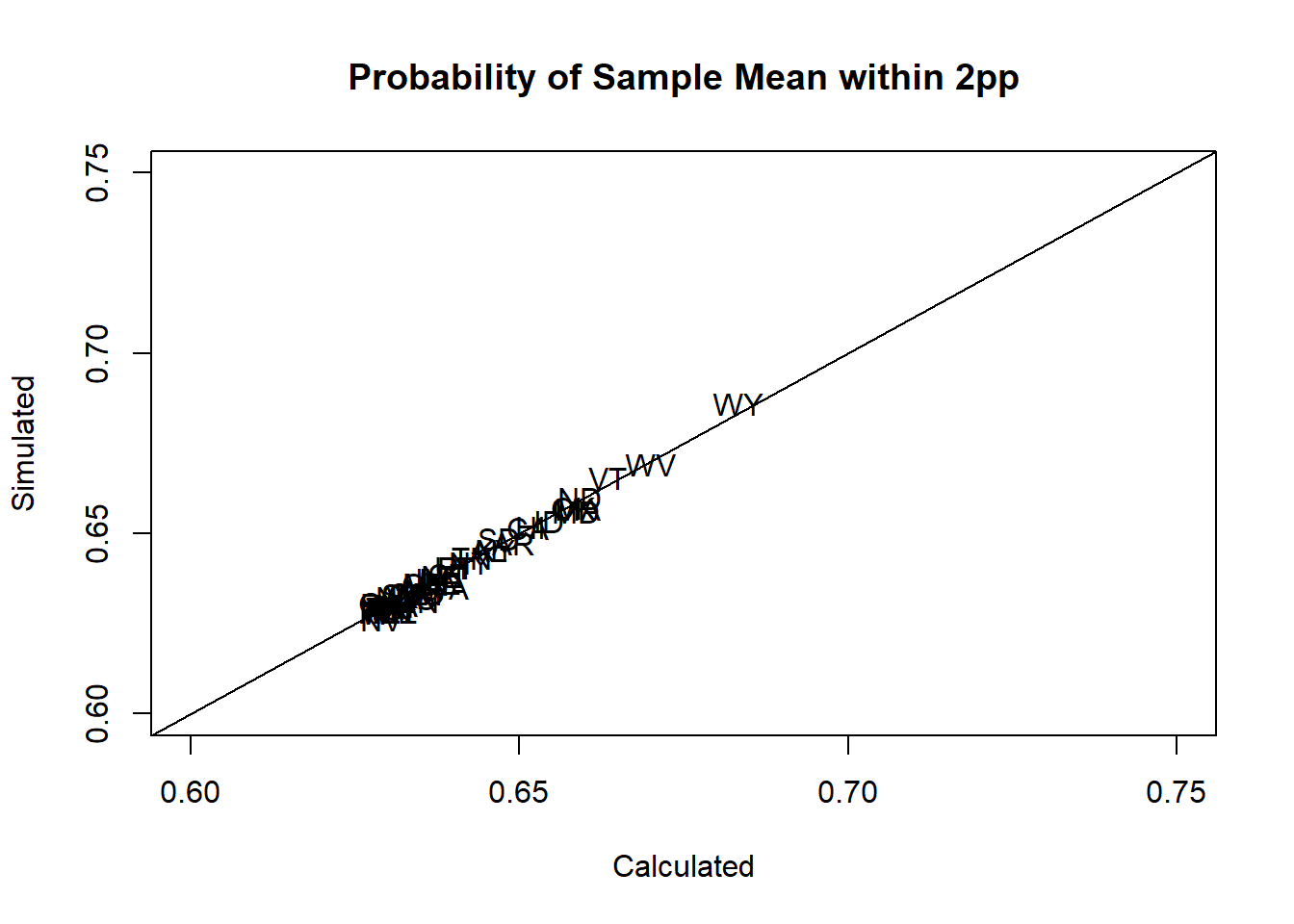
(c) (Bonus) This question is quite hard! Add a final column that, in each state, gives the number of respondents (rounded to the nearest whole number) that would ensure that 99% of all estimates of Biden’s support will be within 1 percentage point of the true value. Simulate drawing an n of this size in each state and show that 99% of estimates fall within those bounds. As a first step, calculate the number of standard deviations above and below the mean in the standard normal distribution that contain 99% of the probability mass. Then think about writing an equation where \(n\) is the only unknown and isolating it.
How many standard deviations in the standard normal contain 99% of all the data?
qnorm(.005)
#> [1] -2.575829
2.57 standard deviations above and below the mean.
Therefore, if
\[ \frac{.01}{se}=-2.57\\ \frac{.01}{\frac{sd_x}{\sqrt{n}}} = -2.57\\ .01*\frac{\sqrt{n}}{sd_x} = -2.57\\ \sqrt{n} = \frac{-2.57*sd_x}{.01}\\ n = (\frac{-2.57*sd_x}{.01})^2 \]
Plugging this in to R
elect$sd <- sqrt(elect$biden.perc *(1-elect$biden.perc))
elect$n.unrounded <- ( (-2.57*elect$sd)/(.01)  )^2
elect$n <- round(elect$n.unrounded)


elect$sim.prop.within.1<- NA

for(i in 1:nrow(elect)){
samp.means <- rbinom(100000,elect$n[i],prob=elect$biden.perc[i])/elect$n[i]

#Test A
elect$sim.prop.within.1[i] <- mean(samp.means>=(elect$biden.perc[i]-.01) & samp.means<=(elect$biden.perc[i]+.01))
}

summary(elect$sim.prop.within.1)
#>    Min. 1st Qu.  Median    Mean 3rd Qu.    Max.
#>  0.9892  0.9897  0.9898  0.9898  0.9900  0.9906
Question 4 (Alternative approach)
Given the nature of the prompt – specifically that i’ve asked you to assess the variability in sample means – the fully correct answers for this question are to consider the sampling distribution used above. That being said, because each sample of 500 people can be thought of as 500 draws from the Bernoulli defined by the biden.perc() column, you get approximately the same answers through assessing the binomial distribution.
- The draw of 500 people will be binomially distributed with a mean that is equal to the population mean. We can determine what proportion of the Binomial distribution is \(\pm 2\%\) from the true population mean.
elect$prop.within.2.bn <- pbinom(500*(elect$biden.perc+.02),size=500, prob=elect$biden.perc) -
pbinom(500*(elect$biden.perc-.02),size=500, prob=elect$biden.perc)- The simulations will be the same as above
plot(elect$prop.within.2.bn, elect$sim.prop.within.2, pch=16, xlab="Calculated",
     ylab="Simulated", main="Probability of Sample Mean within 2pp", type="n")
text(elect$prop.within.2.bn, elect$sim.prop.within.2,elect$state)
abline(0,1)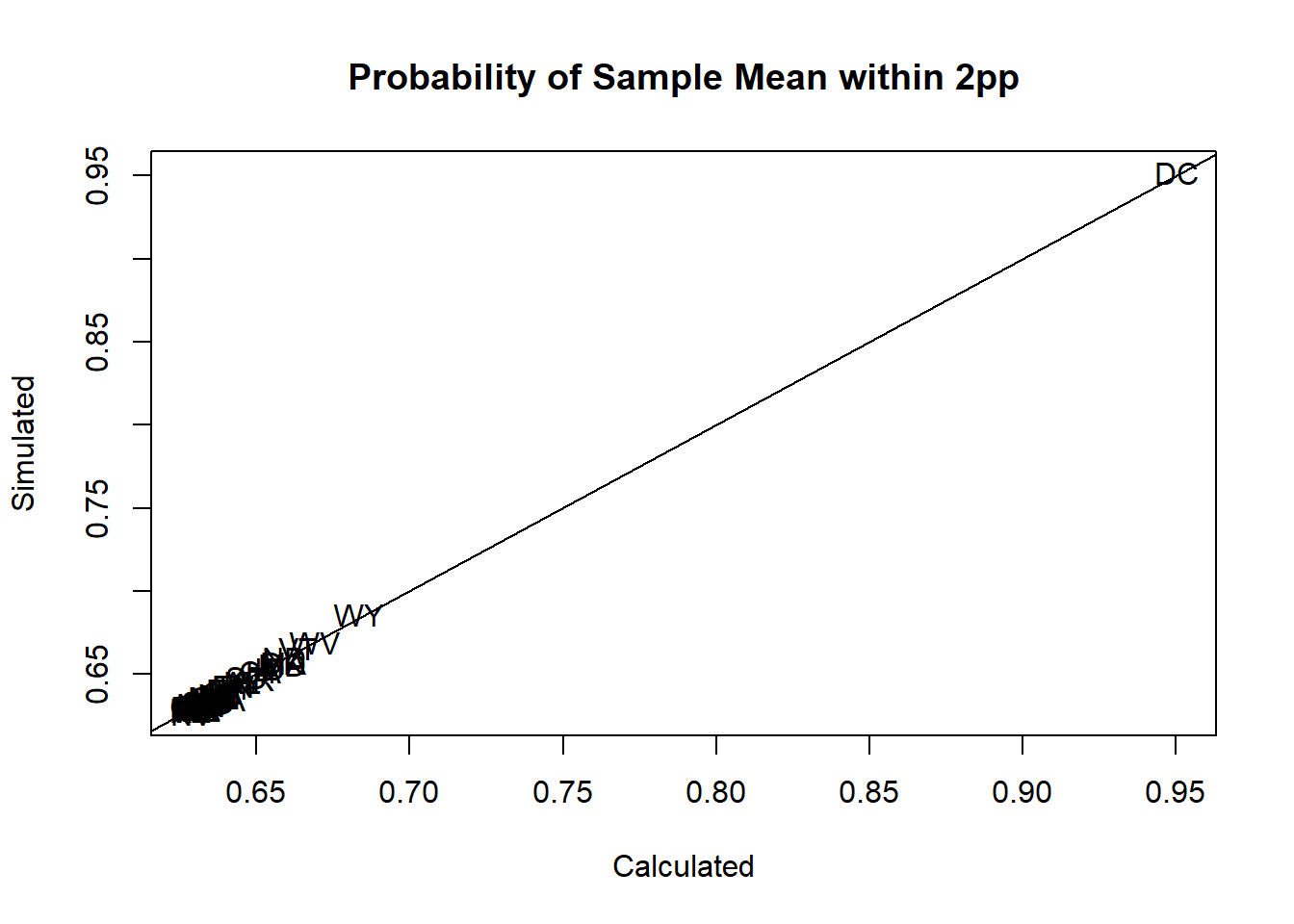
I don’t, as of right now, believe that this question is answerable without using the normal distribution. The above calculation works because we can consider the amount of “standard errors” that contain 99% of the probability distribution for any normal distribution, and solve for \(n\) given that information. There is no “Standard Binomial”, and critically, the shape of the binomial depends on \(\pi\), so we can’t just figure out a set range of “Binomial-Variances” and use that to solve for \(n\). If you were able to estimate the following numbers mathematically, you can get some points for this question:
elect$n
#>  [1] 16329 15411 15178 16512 15044 16194 15826  3452 15900
#> [10] 16493 16512 15020 16397 14847 16017 16069 16141 15361
#> [19] 15921 14577 14597 16368 16499 16425 16107 16048 16047
#> [28] 16509 14554 15880 16419 16082 16311 16502 15606 16402
#> [37] 14617 16056 16510 15770 16280 15320 15588 16459 15757
#> [46] 16337 14301 15862 16512 13923 13174