How the Decision Desk Works
Written by Marc Trussler for the NBC Decision Desk
November 2023
This material will not be assessed.
The task of a decision desk is to determine, with a great deal of accuracy, who is likely to win an election before all the votes are finished counting.
Ideally, we wish to call a race as early as possible. The caveat being we also wish to never call a race incorrectly.
The keys to doing this are:
- Leverage the past.
- Remember that turnout is unknown.
- Know the assumptions of your model (and why they are almost certainly wrong).
The first vote update
We are going to imagine an election an a hypothetical state with 15 different counties. Generally speaking we get data from counties, though sometimes we get data directly from election precincts.
Over the course of an election night we will get updates of votes in those states. Here we will get 18 different updates, but in reality we are likely to get hundreds of updates per state over the course of the night, each triggering a re-calculation of our models.
In this case our job will be made significantly easier by the fact that I generated these data so I know what the “right” answer is that we are looking for. The Democrat is going to win this election with:
58.2% of the vote. But we will proceed naively as if we did not know this information.
Imagine it is shortly after poll close and we get this first update of information from our counties:
dat <- race.updates[[1]]
dat
#>    dem.votes rep.votes complete
#> 1        158       205    FALSE
#> 2          0         0    FALSE
#> 3          0         0    FALSE
#> 4        192      3372    FALSE
#> 5          0         0    FALSE
#> 6          0         0    FALSE
#> 7        400      1561    FALSE
#> 8          0         0    FALSE
#> 9          0         0    FALSE
#> 10         0         0    FALSE
#> 11       954       195    FALSE
#> 12         0         0    FALSE
#> 13       455       281    FALSE
#> 14         0         0    FALSE
#> 15         0         0    FALSE
We have data from only a few counties here. At this point, if I want to determine who is going to win what can I do?
Well, the easiest thing I could do is to figure out what percent the candidates are getting statewide and assume that it is the right number. For simplicity here I will just calculate the democratic percent of the vote, as there are only two candidates in the race. If this number is below 50% we believe the Republican will win and if it is above 50% we believe the Democrat will win.
The democrat is winning 27% of the vote in this vote update.
Let’s say we want to make this our guess of what is going to happen for the rest of the night. What has to be true for that to be a good guess? Thinking about what we’ve learned about sampling, we have learned that the sample mean is an unbiased estimator of a population parameter if we have a random sample of data. In other words, we think estimate is drawn from the sampling distribution surrounding the true population paramater if, and only if, this is a random sample of the votes.
But that’s almost certainly not true!
First, we have a bunch of 0 counties. So we would have to believe that the counties that have vote are perfectly representative of the counties that do not have vote. Further, even within the counties that have vote this might be 5% or 50% or 100% of their vote, so we might have some Republican county making up a disproportionately large amount of the vote we currently have in.
We are going to get 18 updates of votes throughout the night, let’s see how this method (statewide percent) will do in predicting democratic vote share over the course of the night:
statewide.voteshare <- function(dat){
est <- sum(dat$dem.votes)/(sum(dat$dem.votes) + sum(dat$rep.votes))
return(est)
}

statewide.voteshare.est <- rep(NA, 18)

for(i in 1:18){
  dat <- race.updates[[i]]
  statewide.voteshare.est[i] <- statewide.voteshare(dat)
}


plot(1:18, statewide.voteshare.est, type="b", ylim=c(.25,.75),
     pch=16,
     main="Vote Estimation Strategies", col="firebrick")
abline(h=.5822, col="magenta", lty=2)
legend("bottomright","Statewide Average", pch=c(16), col=c("firebrick"))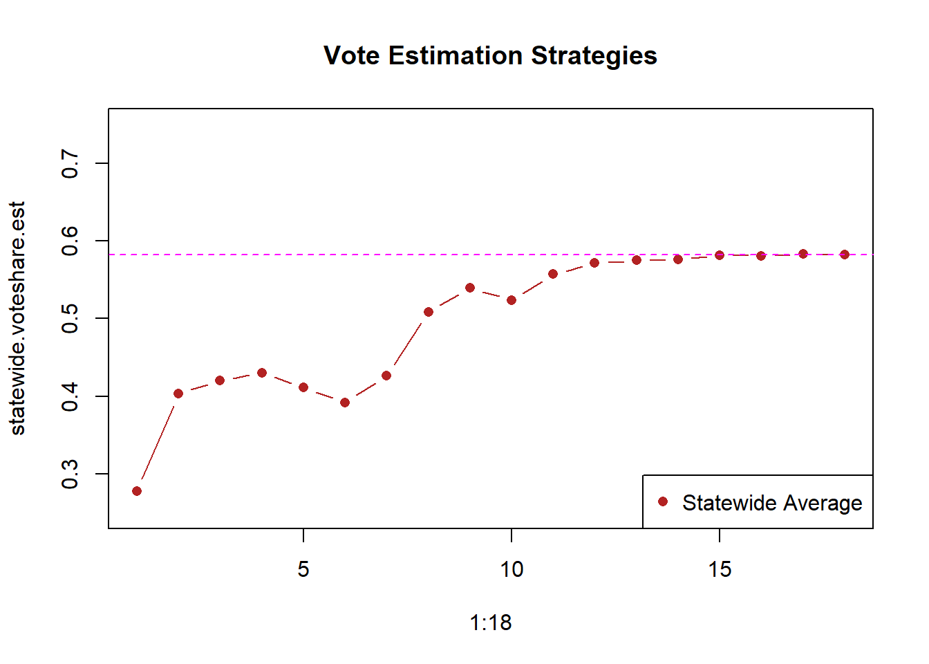
It starts way too low and take a long, long time to get to the right level. It’s really only by update 12 or 13 that this gets to the right level. More-so, the variance in this estimator is huge. We start with a guess of the democrat winning less than 30% of the vote, and end up 28 percentage points higher.
We can do a lot better!
Let’s modify this approach. Right now we are saying that the statewide percent is just correct, but certainly we know more information about the counties that actually have vote reporting.
What if, for those counties, we assume that the vote they are currently getting is representative of the vote they will get the rest of the night. That’s probably more accurate than just assuming every county will get the statewide average:
#Assume that the percent in each county is correct,
#If no vote in a county use statewide percentage
dat <- race.updates[[1]]


dat$pred.dem.perc <- dat$dem.votes/(dat$dem.votes + dat$rep.votes)
dat
#>    dem.votes rep.votes complete pred.dem.perc
#> 1        158       205    FALSE    0.43526171
#> 2          0         0    FALSE           NaN
#> 3          0         0    FALSE           NaN
#> 4        192      3372    FALSE    0.05387205
#> 5          0         0    FALSE           NaN
#> 6          0         0    FALSE           NaN
#> 7        400      1561    FALSE    0.20397756
#> 8          0         0    FALSE           NaN
#> 9          0         0    FALSE           NaN
#> 10         0         0    FALSE           NaN
#> 11       954       195    FALSE    0.83028721
#> 12         0         0    FALSE           NaN
#> 13       455       281    FALSE    0.61820652
#> 14         0         0    FALSE           NaN
#> 15         0         0    FALSE           NaN
Now for the remaining counties, we can just fill in the statewide average (which right now is 27%):
statewide <- sum(dat$dem.votes)/(sum(dat$dem.votes) + sum(dat$rep.votes))
dat$pred.dem.perc[is.nan(dat$pred.dem.perc)] <- statewide
dat
#>    dem.votes rep.votes complete pred.dem.perc
#> 1        158       205    FALSE    0.43526171
#> 2          0         0    FALSE    0.27775634
#> 3          0         0    FALSE    0.27775634
#> 4        192      3372    FALSE    0.05387205
#> 5          0         0    FALSE    0.27775634
#> 6          0         0    FALSE    0.27775634
#> 7        400      1561    FALSE    0.20397756
#> 8          0         0    FALSE    0.27775634
#> 9          0         0    FALSE    0.27775634
#> 10         0         0    FALSE    0.27775634
#> 11       954       195    FALSE    0.83028721
#> 12         0         0    FALSE    0.27775634
#> 13       455       281    FALSE    0.61820652
#> 14         0         0    FALSE    0.27775634
#> 15         0         0    FALSE    0.27775634
This is a more nuanced picture of the election.
Ok, but, what is our overall guess at the statewide democratic percent with these data? Is it this:
mean(dat$pred.dem.perc)
#> [1] 0.3279446
No! Counties don’t vote! People do! This assumes that all of these counties are equally sized, which is probably not true.
This leads to the first major wrinkle of election forecasting. It’s not just about predicting the percentage in every county, we have to predict turnout too. That is, after we estimate candidate percents, we need to multiply that by how many people those percentages actually represent.
It’s not just as easy as saying: well let’s take a weighted mean of these percentages based on the number of registered voters. That would assume that the proportion who turnout in each county will be equal, and that’s not true! Where people are turning out is a big part of the election dynamics.
So we need an estimate of the total number of voters expected in each county. Where might this number come from? Well to start: we make it up! Here let’s say we think that turnout will be a bit lower in this cycle than the previous. We might start with something like:
dat$expected.vote <- round(truth$past.votes*.95)
dat$est.dem.votes <- dat$pred.dem.perc*dat$expected.vote
Why do we just guess? Well, what else are we going to do?? The guess is an educated one, and we can talk more about some things we’ve done to tighten that estimate, but ultimately how would we know how many people are going to show up to vote?
So with that we have enough info to build method two, which I’ll call statewide.corrected. Again, we are saying that if a county has vote we will assume that the percent is correct. If a county doesn’t have vote we will use the statewide average as what we expect from that state:
statewide.corrected <- function(dat){

dat$pred.dem.perc <- dat$dem.votes/(dat$dem.votes + dat$rep.votes)
statewide <- sum(dat$dem.votes)/(sum(dat$dem.votes) + sum(dat$rep.votes))
dat$pred.dem.perc[is.nan(dat$pred.dem.perc)] <- statewide
dat$expected.vote <- truth$past.votes*.95
dat$est.dem.votes <- dat$pred.dem.perc*dat$expected.vote

est <- sum(dat$est.dem.votes)/sum(dat$expected.vote)
return(est)
}

statewide.corrected.est <- rep(NA, 18)

for(i in 1:18){
  dat <- race.updates[[i]]
  statewide.corrected.est[i] <- statewide.corrected(dat)
}


plot(1:18, statewide.voteshare.est, type="b", ylim=c(.25,.75),
     pch=16,
     main="Vote Estimation Strategies", col="firebrick")
points(1:18, statewide.corrected.est, type="b", pch=16, col="darkorange")
abline(h=.5822, col="magenta", lty=2)
legend("bottomright","Statewide Average", pch=c(16,16), col=c("firebrick","darkorange"))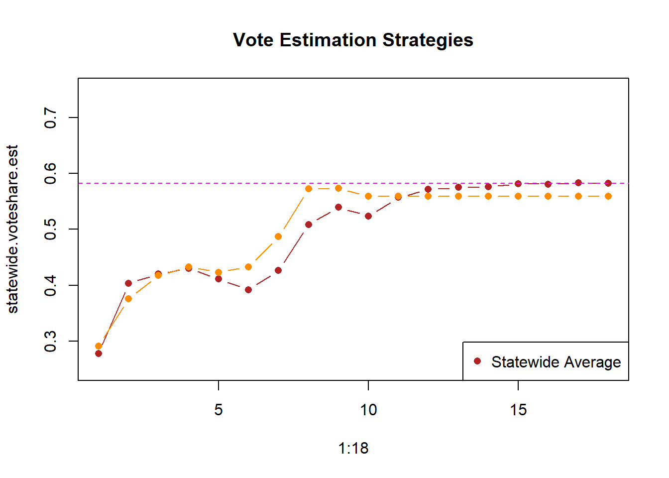
This does marginally better, particularly in the mid part of the night. After about update 8 we are pretty close to the right answer. But that’s still pretty late, and we still have way more variance then I would like.
Using the past
The big change that we can make – and this is one of the key insights of election forecasting – is that we can use the past relationships between counties to make predictions about counties that have no vote.
If we think about the first update of information that we get, where we had a bunch of counties that had 0s do we really have no information about those places? Of course not! We know what has happened in the recent past in those places.
Take Philadelphia county, for example. We know that Democratic candidates win around 80-90% of the vote in Philadelphia. If we have no vote in Philadelphia should we throw up our hands and say: I don’t know! Whatever the statewide percent of the vote is, that’s fine! Of course not. We know that Philadelphia will be an overwhelmingly democratic county.
So in this case, we have the past democratic percent in each place:
dat <- race.updates[[1]]

cbind.data.frame(dat, truth$past.dem.percents)
#>    dem.votes rep.votes complete truth$past.dem.percents
#> 1        158       205    FALSE              0.42997942
#> 2          0         0    FALSE              0.73951339
#> 3          0         0    FALSE              0.76239682
#> 4        192      3372    FALSE              0.05442398
#> 5          0         0    FALSE              0.41159660
#> 6          0         0    FALSE              0.88465222
#> 7        400      1561    FALSE              0.19843429
#> 8          0         0    FALSE              0.33452472
#> 9          0         0    FALSE              0.38477784
#> 10         0         0    FALSE              0.20492551
#> 11       954       195    FALSE              0.71452458
#> 12         0         0    FALSE              0.86992537
#> 13       455       281    FALSE              0.62185867
#> 14         0         0    FALSE              0.79694469
#> 15         0         0    FALSE              0.52870303
Our first inclination might be: well let’s use those past dem percents anywhere we have a 0. So in county 2 we might fill in that the predicted dem percent is 73.9% of the vote.
But we can do better than that! For one thing, such a model would assume that every election will have the same outcome. But why not just skip all the modelling and say: the democratic candidate will get the same percent of the vote as the previous democratic candidate. That’s real lazy, and doesn’t allow for elections to actually change anything.
To step out of our simulation for a moment, look at the county level relationship between the percent each county in PA voted for Biden for President in 2020 (x-axis), and for Shapiro for Governor in 2022 (y-axis).
library(rio)
pa <- import("https://github.com/marctrussler/IIS-Data/raw/main/PAElectionResults.Rds")

plot(pa$biden.pct, pa$shapiro.pct, pch=16, ylim=c(0,1), xlim=c(0,1),
     xlab="Biden", ylab="Shapiro",
     main="PA 2020-2022 Vote Shift")
abline(lm(pa$shapiro.pct ~ pa$biden.pct), col="firebrick", lty=2)
abline(0,1)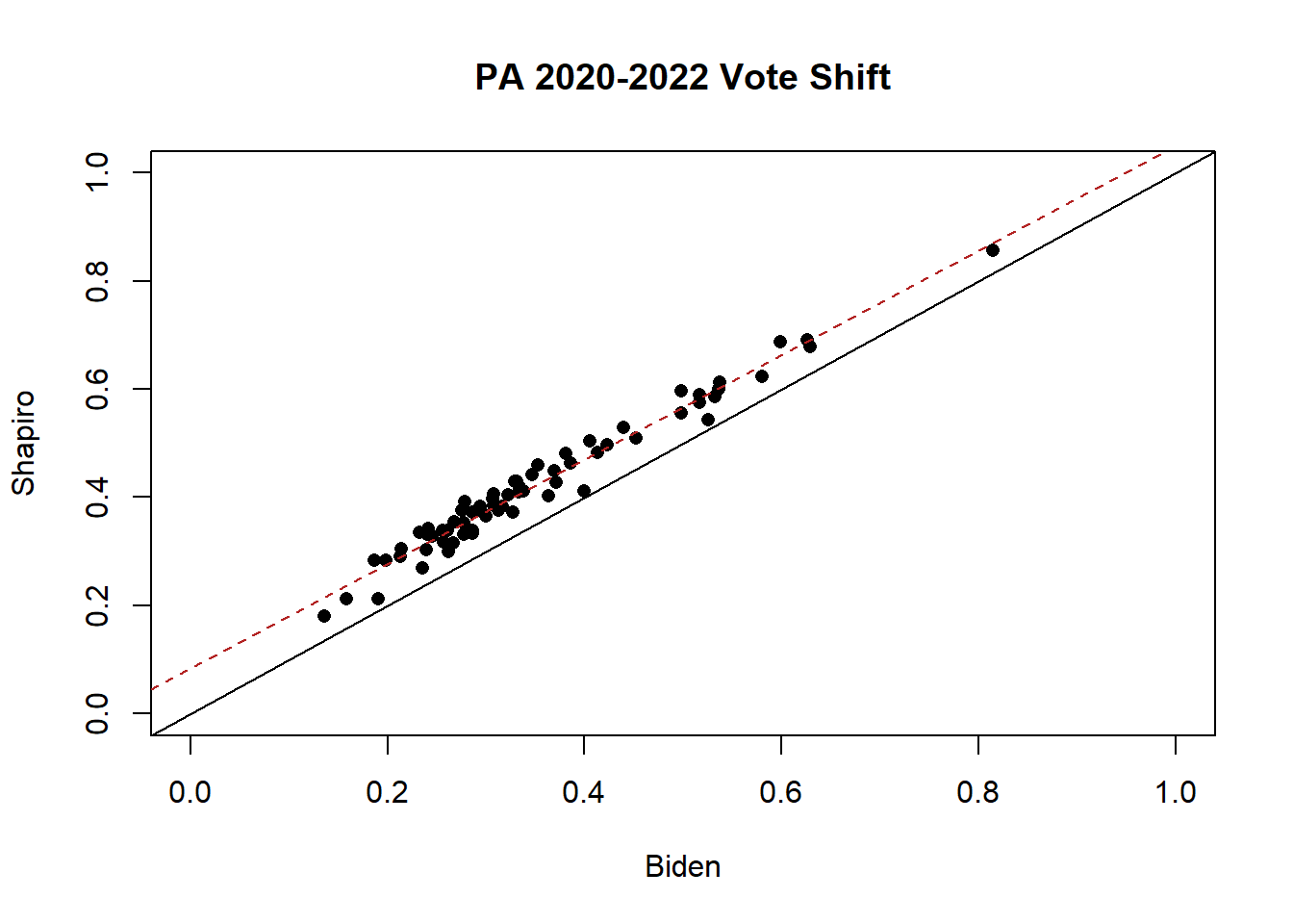
mean(pa$biden.pct - pa$shapiro.pct)
#> [1] -0.07161698
If all the points were on the black line, that would mean that Shapiro got the exact same percent of the vote as Biden in all of these locations. That’s not what we see, however, all the black points are above the line, indicating that Shapiro out-performed Biden in all of these locations.
But the over-performance is relatively uniform. The relationships between all the counties stayed relatively constant. Shapiro just shifted Biden’s vote share around 7 percentage points in all places. This isn’t a perfect relationship – some shifted a bit more and some shifted a bit less – but overall, it is pretty remarkable that a uniform shift took place in the state.
We can apply this same logic to our fake election we are running here.
Looking at that first update, we can ask: for counties that have some vote, how much has the democratic percentage shifted relative to the previous race?
dat$pred.dem.perc <- dat$dem.votes/(dat$dem.votes + dat$rep.votes)
dat <- cbind.data.frame(dat, truth$past.dem.percents)
dat
#>    dem.votes rep.votes complete pred.dem.perc
#> 1        158       205    FALSE    0.43526171
#> 2          0         0    FALSE           NaN
#> 3          0         0    FALSE           NaN
#> 4        192      3372    FALSE    0.05387205
#> 5          0         0    FALSE           NaN
#> 6          0         0    FALSE           NaN
#> 7        400      1561    FALSE    0.20397756
#> 8          0         0    FALSE           NaN
#> 9          0         0    FALSE           NaN
#> 10         0         0    FALSE           NaN
#> 11       954       195    FALSE    0.83028721
#> 12         0         0    FALSE           NaN
#> 13       455       281    FALSE    0.61820652
#> 14         0         0    FALSE           NaN
#> 15         0         0    FALSE           NaN
#>    truth$past.dem.percents
#> 1               0.42997942
#> 2               0.73951339
#> 3               0.76239682
#> 4               0.05442398
#> 5               0.41159660
#> 6               0.88465222
#> 7               0.19843429
#> 8               0.33452472
#> 9               0.38477784
#> 10              0.20492551
#> 11              0.71452458
#> 12              0.86992537
#> 13              0.62185867
#> 14              0.79694469
#> 15              0.52870303
shift <- mean(truth$past.dem.percents - dat$pred.dem.perc, na.rm=T)
shift
#> [1] -0.02447682
The counties that have votes have shifted 2.4 points less democratic compared to the previous race.
Now, we can apply that same shift to the counties that don’t have any votes:
dat$pred.dem.perc[is.nan(dat$pred.dem.perc)] <- truth$past.dem.percents[is.nan(dat$pred.dem.perc)] + shift
dat
#>    dem.votes rep.votes complete pred.dem.perc
#> 1        158       205    FALSE    0.43526171
#> 2          0         0    FALSE    0.71503657
#> 3          0         0    FALSE    0.73792000
#> 4        192      3372    FALSE    0.05387205
#> 5          0         0    FALSE    0.38711977
#> 6          0         0    FALSE    0.86017539
#> 7        400      1561    FALSE    0.20397756
#> 8          0         0    FALSE    0.31004789
#> 9          0         0    FALSE    0.36030102
#> 10         0         0    FALSE    0.18044869
#> 11       954       195    FALSE    0.83028721
#> 12         0         0    FALSE    0.84544854
#> 13       455       281    FALSE    0.61820652
#> 14         0         0    FALSE    0.77246786
#> 15         0         0    FALSE    0.50422621
#>    truth$past.dem.percents
#> 1               0.42997942
#> 2               0.73951339
#> 3               0.76239682
#> 4               0.05442398
#> 5               0.41159660
#> 6               0.88465222
#> 7               0.19843429
#> 8               0.33452472
#> 9               0.38477784
#> 10              0.20492551
#> 11              0.71452458
#> 12              0.86992537
#> 13              0.62185867
#> 14              0.79694469
#> 15              0.52870303
And now that we have democratic percentages in each location, we can apply those to our turnout estimates and get an estimate for what we think is going to happen in the race overall.
Let’s apply that model to all of the race updates:
shift.model <- function(dat){
dat$pred.dem.perc <- dat$dem.votes/(dat$dem.votes + dat$rep.votes)
shift <- mean(truth$past.dem.percents - dat$pred.dem.perc, na.rm=T)
dat$pred.dem.perc[is.nan(dat$pred.dem.perc)] <- truth$past.dem.percents[is.nan(dat$pred.dem.perc)] + shift
dat$expected.vote <- truth$past.votes*.95
dat$est.dem.votes <- dat$pred.dem.perc*dat$expected.vote

est <- sum(dat$est.dem.votes)/sum(dat$expected.vote)
return(est)
}

shift.model.est <- rep(NA, 18)

for(i in 1:18){
  dat <- race.updates[[i]]
  shift.model.est[i] <- shift.model(dat)
}


plot(1:18, statewide.voteshare.est, type="b", ylim=c(.25,.75),
     pch=16,
     main="Vote Estimation Strategies", col="firebrick")
points(1:18, statewide.corrected.est, type="b", pch=16, col="darkorange")
points(1:18, shift.model.est, type="b", pch=16, col="forestgreen")
abline(h=.5822, col="magenta", lty=2)
legend("bottomright","Statewide Average", pch=c(16,16,16), col=c("firebrick","darkorange","forestgreen"))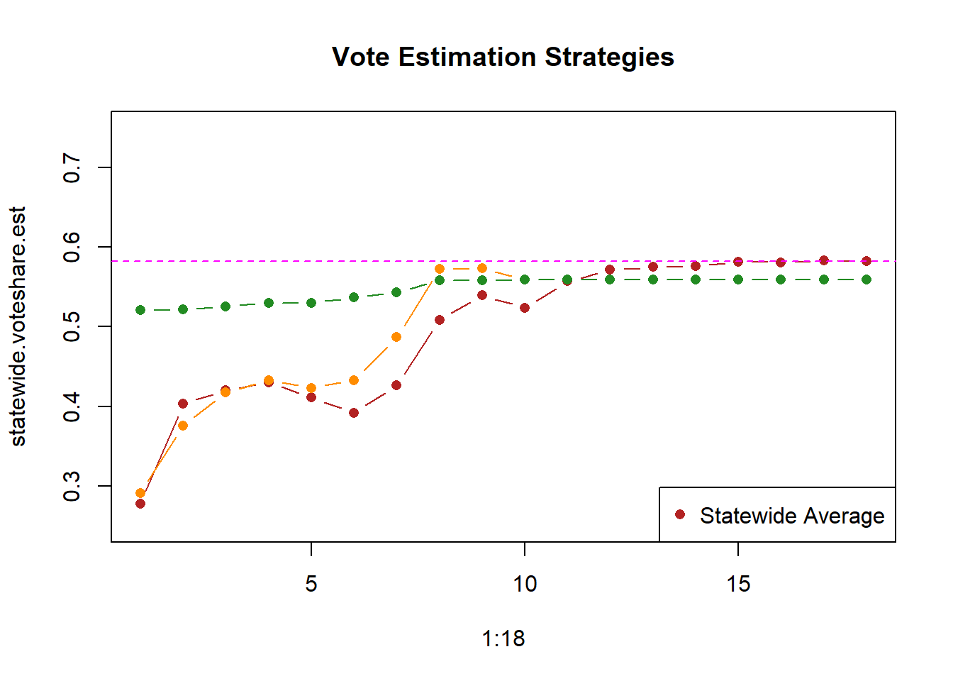
Look how much better this did! It’s not perfect: the data that we have at the start is not perfectly representative and shifts are not perfectly uniform across counties, so we start a little bit low. But we are in the ballpark the whole time.
By leveraging the fact that elections are not independent, we can use a shift model to orient us in the approximately correct place much earlier.
Fixing Turnout
OK, so we have a method that works pretty well, but the green dots are lining up exactly with the truth…. why not? Well remember that we had to estimate turnout, and as of right now that estimation is just “Eh, turnout will be 95% of the previous race”. That’s not very sophisticated, and may or may not end up with the right number.
The last step we can do here is to improve the estimation of turnout as our night goes on.
To do so, we are goign to use the column we haven’t touched yet, called complete.
As long as counties are still counting their vote, we have no real idea how many votes will be counted in that place. We can guess – based on how many precincts have completed, or previous trends in how they counted, or based on interviews and phone calls with officials – but those are all just guesses.
However, when a county tells us “Hey, we are finished counting our votes!” that’s real, concrete information on turnout.
The last thing we want to do is to leverage that information about complete counties to influence our turnout estimate.
To do so, we are going to do something very similar to what we did above for the shift model. When a county is complete, we are going to determine what their turnout is as a percentage of the previous election turnout. Then, instead of saying “We think turnout is going to be 95% of the previous election” (a guess!), we can say “We think turnout in non complete counties is goign to be the same percentage of the previous election as it is in the completed counties.”
So let’s go to an update that has some complete counties:
dat <- race.updates[[12]]
dat
#>    dem.votes rep.votes complete
#> 1       3140      4083    FALSE
#> 2       8298      2985    FALSE
#> 3      26214      6958    FALSE
#> 4       1325     23310    FALSE
#> 5       3722      5079    FALSE
#> 6      10673       586    FALSE
#> 7       5432     21178    FALSE
#> 8       2315      3796     TRUE
#> 9      11801     18337     TRUE
#> 10      1586      6095    FALSE
#> 11     13220      2698     TRUE
#> 12     14799       648    FALSE
#> 13      6563      4059    FALSE
#> 14     33004      6412     TRUE
#> 15      8596      6916    FALSE
For the completed counties, what is the turnout relative to the past race?
turnout.percent <- (dat$dem.votes[dat$complete] +dat$rep.votes[dat$complete])/truth$past.votes[dat$complete]
turnout.percent
#> [1] 0.6980011 0.6814852 0.8784283 0.9061566
Let’s use that information to form a new estimate of turnout, relative to the previous race:
turnout.ratio <- mean(turnout.percent)
turnout.ratio
#> [1] 0.7910178
Much lower than we thought initially! That happens!
Now we can apply this better informed estimate of the turnout ratio:
dat$expected.vote.old <- truth$past.votes*.95
dat$expected.vote.new <- truth$past.votes*turnout.ratio
Let’s add that step to our model and see what happens. (I don’t want to get bogged down in details, but specifically here i’m applying that ratio only after we have three complete counties, and i’m not applying it to counties that are already complete. We don’t have to estimate turnout for those counties.)
shift.model.turnout <- function(dat){
dat$pred.dem.perc <- dat$dem.votes/(dat$dem.votes + dat$rep.votes)
shift <- mean(truth$past.dem.percents - dat$pred.dem.perc, na.rm=T)
dat$pred.dem.perc[is.nan(dat$pred.dem.perc)] <- truth$past.dem.percents[is.nan(dat$pred.dem.perc)] + shift

#Turnout estimation
if(sum(dat$complete)>=3){
turnout.percent <- (dat$dem.votes[dat$complete] +dat$rep.votes[dat$complete])/truth$past.votes[dat$complete]
turnout.ratio <- mean(turnout.percent)
dat$expected.vote <- truth$past.votes*turnout.ratio
dat$expected.vote[dat$complete] <- dat$dem.votes[dat$complete] + dat$rep.votes[dat$complete]
} else{
dat$expected.vote <- truth$past.votes*.95
}

dat$est.dem.votes <- dat$pred.dem.perc*dat$expected.vote
est <- sum(dat$est.dem.votes)/sum(dat$expected.vote)
return(est)
}

shift.model.turnout.est <- rep(NA, 18)

for(i in 1:18){
  dat <- race.updates[[i]]
  shift.model.turnout.est[i] <- shift.model.turnout(dat)
}


plot(1:18, statewide.voteshare.est, type="b", ylim=c(.25,.75),
     pch=16,
     main="Vote Estimation Strategies", col="firebrick")
points(1:18, statewide.corrected.est, type="b", pch=16, col="darkorange")
points(1:18, shift.model.est, type="b", pch=16, col="forestgreen")
points(1:18, shift.model.turnout.est, type="b", pch=16, col="black")

abline(h=.5822, col="magenta", lty=2)
legend("bottomright",c("Statewide Average", "Statwide Average Corrected", "Shift", "Shift + Turnout"), pch=c(16,16,16,16), col=c("firebrick","darkorange","forestgreen", "black"))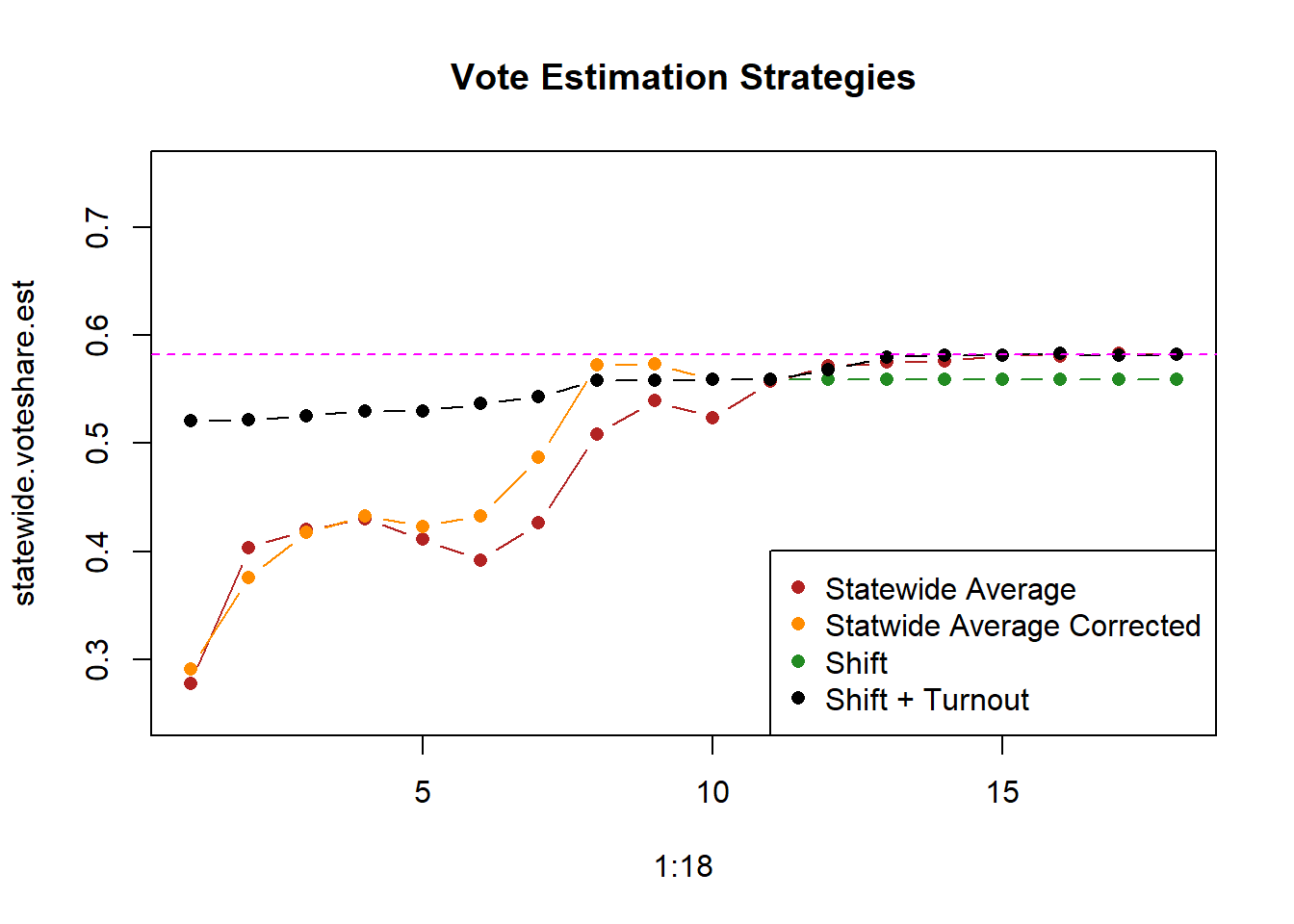
Until we have complete counties the Shift and Shift+Turnout are exactly the same. Once we start getting complete counties the turnout model kicks in and that model starts to do a better job of nailing the final answer.
Assumptions
In order for us to be able to make calls with a model like this we need to know what assumptions are needed to trust the results. Here are the two big ones:
The first important assumption is that the shift that takes place from the past race is uniform for all counties in a state. Looking at the Pennsylvania reports above, that looks like a pretty good assumption, but we could imagine times where that would not be true. Where certain types of counties shift more or less than others. (For example in the 2020 election suburban counties shifted a lot, but rural counties did not).
To relax this assumption we actually split states into several micro-states we call “strata”. These strata are organized either by partisanship (put all the High Democratic states together) or by geography (put all the Philadelphia suburbs together), and then we estimate and apply the shifts within those strata. Those same strata are applied at the turnout step so that different areas can have a turnout pattern that’s seperate from the rest of the state.
The second important assumption is that the votes that are reported in a county are representative of what is to come in that county. In the model we used above the shifts were only applied to counties with 0 votes. Once a county got votes we assumed that all the votes within the county would be allocated with the same percent.
Why might that be wrong?
Two big reasons: (1) Geographic un-eveness in reporting; (2) Mode effects.
For the first imagine if the precincts in the far NE of Philadelphia were the first to report. These precincts are the most Republican, and as such it would give the false impression that Philadelphia would be way more Republican than it actually would end up as.
There is not much to be done about this problem other than a bit of investigative work (looking at county websites) to see what precincts have reported. But sometimes you just have to wait! We are very skeptical if a county shifts a huge amount from their prior vote.
Mode effects are also a reason to be concerned. We know that, particularly post 2020, Republicans are much more likely to vote in person and Democrats are more likely to vote early or by mail. Most places will not report the votes out in a random order. You might get all the mail votes first, or they may not open the mail until the next day. This will obviously break a model that thinks that the votes in a county are representative of what’s to come!
The solution here is to effectively treat each county-mode as it’s own county. So in Arizona, for example, we would think of Maricopa-Mail as a separate county from Maricopa-Eday. The model would then make the more reasonable assumption that votes within a county-mode are representative of what’s to come.
(Even this has it’s own problem. First: the data quality for these mode-splits are horrendous and filled with errors. The models we built to work with this data worked in maybe 3 states. Second: the assumption that votes within a county-mode are representative of what’s to come is why Fox News called Arizona too early in 2020. Actually because of Maricopa.)
Sampling Distribution?
An additional consideration to make is whether, at any given time, we can think about whether we can put a confidence interval around the estimate we are making.
We have learned that the CLT tells us that we can form a confidence interval by using the formula:
\[ CI(\alpha) = [\bar{X_n} - t_{n-1}(\alpha/2)*\frac{s}{\sqrt{n}},\bar{X_n} + t_{n-1}(\alpha/2)*\frac{s}{\sqrt{n}} ] \]
Is this an appropriate thing to apply to the estimates we are making here?
Well, ignoring the fact that we aren’t really taking means to generate our estimates, more importantly this relies on what we have being a random sample. That’s at the center of everything we did. And we just saw that it’s not a random sample!
Instead of relying on the central limit theorem, we rely on the basic idea of sampling distributions that it is the distribution of all possible estimates if we repeatedly sampled the same data repeatedly.
We can’t come up with a math equation to generate a sampling distribution, but we do have a long, long history of elections.
So what we do instead of analytically deriving a sampling distribution is run our models on old data and ask, for any given point in the night how far is the estimate we are forming from the truth in that race? This gives us an idea of how much error in our estimate there has historically been.
We can re-generate the election day we were using above a large number of times to see what this might look like. (See R file for the code, which i’ve suppressed here).
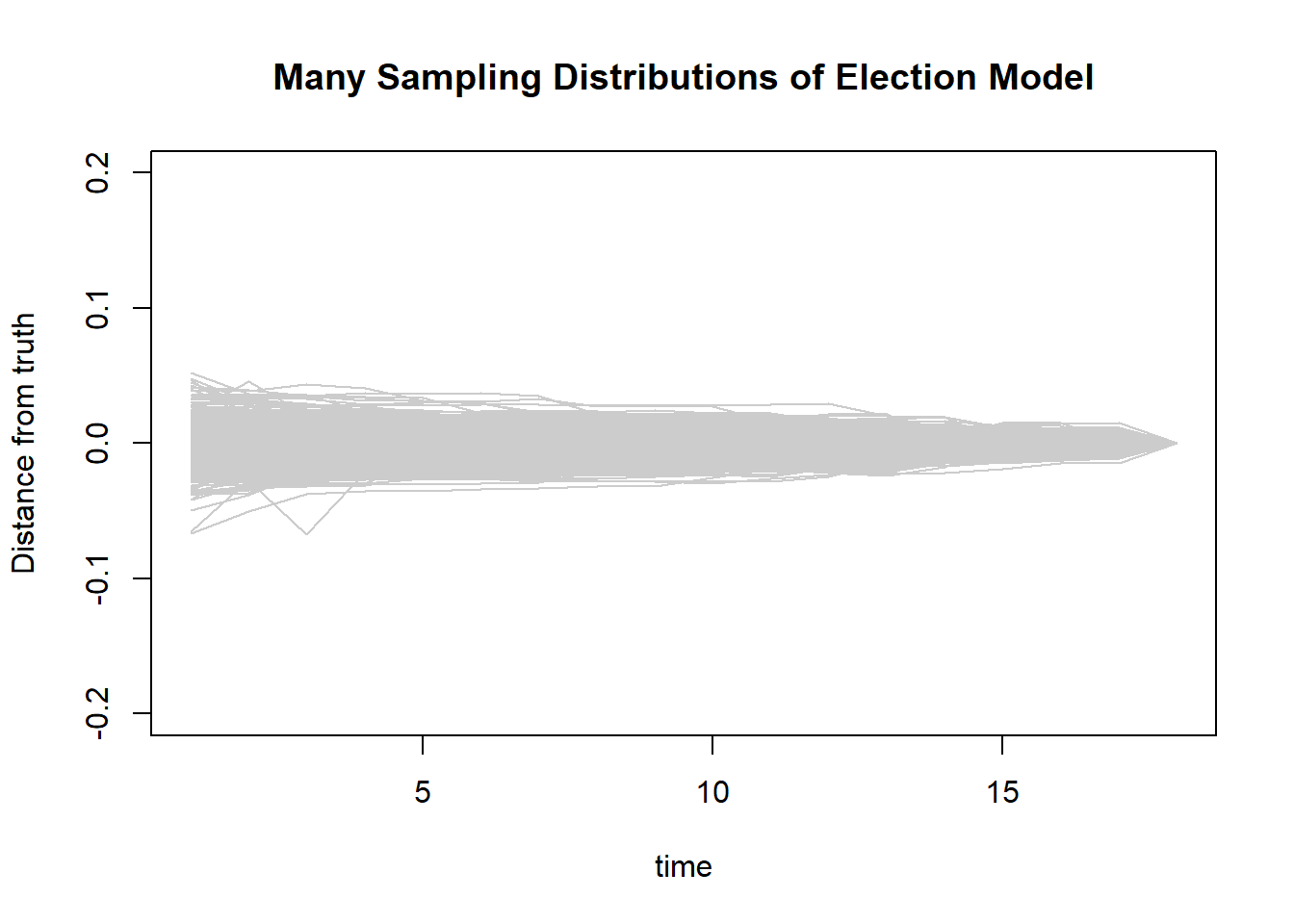
Here are 500 runs of our election model on new data each time. At each time point we are asking: how far is our estimate of the margin away from the truth?
We see that (as expected) early on we are further off, but as more data comes in our estimate gets closer to the truth.
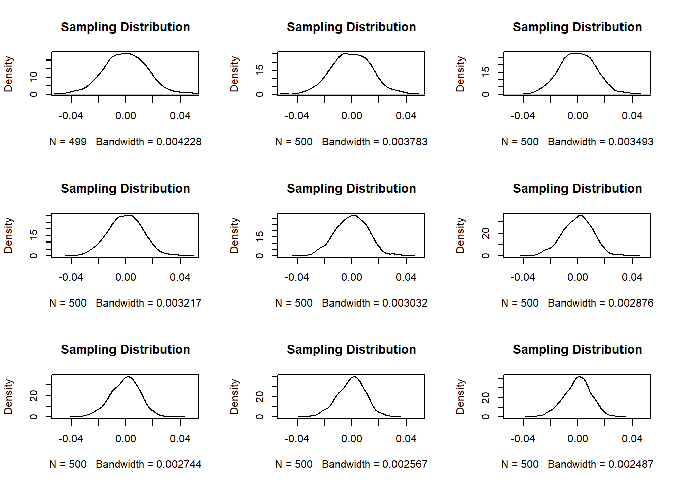
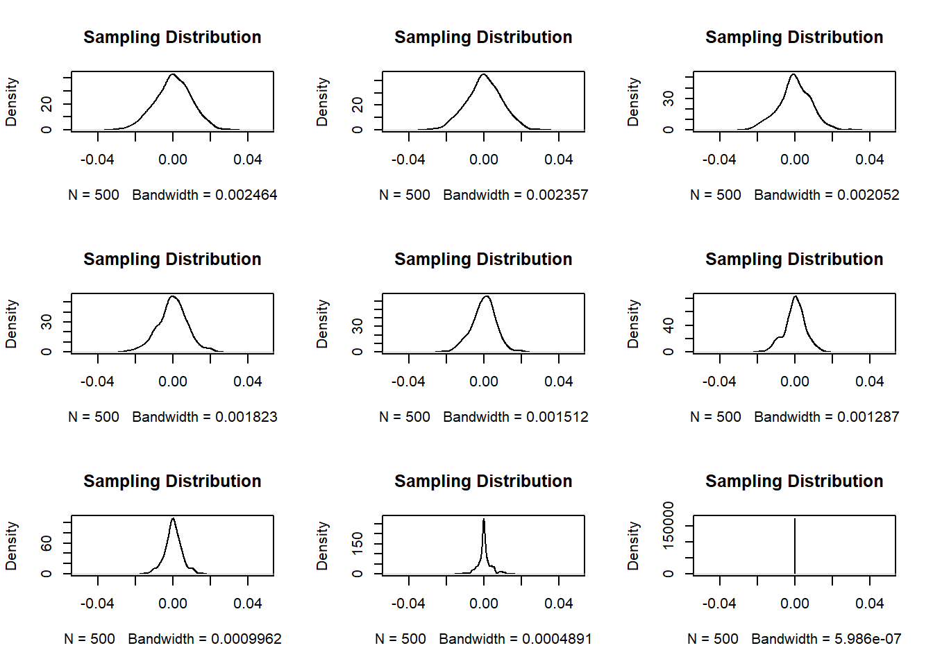
We could then estimate what the shape and standard deviation of this distribution is at many given points:
par(mfrow=c(3,3))
se <- rep(NA, 4)
for(i in 1:nrow(results.matrix)){
  plot(density(results.matrix[i,],na.rm=T), main="Sampling Distribution", xlim=c(-.05,.05))
  se[i] <- sd(results.matrix[i,],na.rm=T)
}
se
#>  [1] 1.645479e-02 1.456725e-02 1.345272e-02 1.238816e-02
#>  [5] 1.167586e-02 1.107471e-02 1.056654e-02 1.003005e-02
#>  [9] 9.784933e-03 9.622277e-03 9.272512e-03 8.539756e-03
#> [13] 7.757782e-03 6.414160e-03 5.560371e-03 4.527146e-03
#> [17] 3.399072e-03 2.521015e-06
These standard deviations can then be used as a pseudo- standard error for our models.