4.5 Distributions of transformations of random variables

Recall that a function of a random variable is also a random variable. If $X$ is a random variable, then $Y=g(X)$ is also a random variable and so it has a probability distribution. Unless $g$ represents a linear rescaling, a transformation will change the shape of the distribution. So the question is: what is the distribution of $g(X)$? We’ll focus on transformations of continuous random variables, in which case the key to answering the question is to work with cdfs.

Example 4.22 Recall the example in Section 3.8.2. Let $U$ be a random variable with a Uniform(0, 1) distribution, and let $X=-\log(1-U)$. We approximated the distribution of $X$ via simulation, and we saw some example calculations in Example 3.15 justifying why the distribution looks like it does. Now we will derive the pdf of $X$.

1. Identify the possible values of $X$. (We have done this already, but this should always be your first step.)
2. Let $F_X$ denote the cdf of $X$. Find $F_X(1)$.
3. Find $F_X(2)$.
4. Find the cdf $F_X(x)$.
5. Find the pdf $f_X(x)$.
6. Why should we not be surprised that $X=-\log(1-U)$ has cdf $F_X(x) = 1 - e^{-x}$? Hint: what is the function $u\mapsto -\log(1-u)$ in this case?

Solution. to Example 4.22

Show/hide solution

1. As always, first determine the range of possible values. When $u=0$, $-\log(1-u)=0$, and as $u$ approaches 1, $-\log(1-u)$ approaches $\infty$; see the picture of the function below. So $X$ takes values in $[0, \infty)$.
2. $F_X(1) = \textrm{P}(X \le 1)$, a probability statement involving $X$. Since we know the distribution of $U$, we express the event $\{X \le 1\}$ as an equivalent event involving $U$.
   $$\{X \le 1\} = \{-\log(1-U) \le 1\} = \{U \le 1 - e^{-1}\}$$ The above follows since $-\log(1-u)\le 1$ if and only if $u\le 1-e^{-1}$; see Figure 4.9 below. Therefore $$F_X(1) = \textrm{P}(X \le 1) = \textrm{P}(-\log(1-U)\le 1) = \textrm{P}(U\le 1-e^{-1})$$ Now since $U$ has a Uniform(0, 1) distribution, $\textrm{P}(U\le u)=u$ for $0<u<1$. The value $1-e^{-1}\approx 0.632$ is just a number between 0 and 1, so $\textrm{P}(U\le 1-e^{-1}) = 1-e^{-1}\approx 0.632$. Therefore $F_X(1)=1-e^{-1}\approx 0.632$. (This is represented in Figure 3.11 by the area of the region from 0 to 1, 63.2%.)
3. Similar to the previous part $$F_X(2) = \textrm{P}(X \le 2) = \textrm{P}(-\log(1-U)\le 2) = \textrm{P}(U\le 1-e^{-2}) = 1-e^{-2}\approx 0.865$$
4. As suggested in the paragraph before the example, the key to finding the pdf is to work with cdfs. We basically repeat the calculation in the previous steps, but for a generic $x$ instead of 1 or 2. Consider $0\le x<\infty$; we wish to find the cdf evaluated at $x$. $$F_X(x) = \textrm{P}(X \le x) = \textrm{P}(-\log(1-U)\le x) = \textrm{P}(U \le 1-e^{-x}) = 1-e^{-x}$$ The above follows since, for $0<x<\infty$, $-\log(1-u)\le x$ if and only if $u\le 1-e^{-x}$; see Figure 4.9 below (illustrated for $x=1$). Now since $U$ has a Uniform(0, 1) distribution, $\textrm{P}(U\le u)=u$ for $0<u<1$. For a fixed $0<x<\infty$, the value $1-e^{-x}$ is just a number between 0 and 1, so $\textrm{P}(U\le 1-e^{-x}) = 1-e^{-x}$. Therefore $F_X(x)=1-e^{-x}, 0<x<\infty$.
5. Differentiate the cdf with respective to $x$ to find the pdf. $$f_X(x) = F'(x) =\frac{d}{dx}(1-e^{-x}) = e^{-x}, \qquad 0<x<\infty$$ Thus we see that $X$ has the pdf in Example 4.14.
6. The function $Q_X(u) = -\log(1-u)$ is the quantile function (inverse cdf) corresponding to the cdf $F_X(x) = 1-e^{-x}$. Therefore, since $U$ has a Uniform(0, 1) distribution, the random variable $Q_X(U)$ will have cdf $F_X$ be universality of the Uniform.

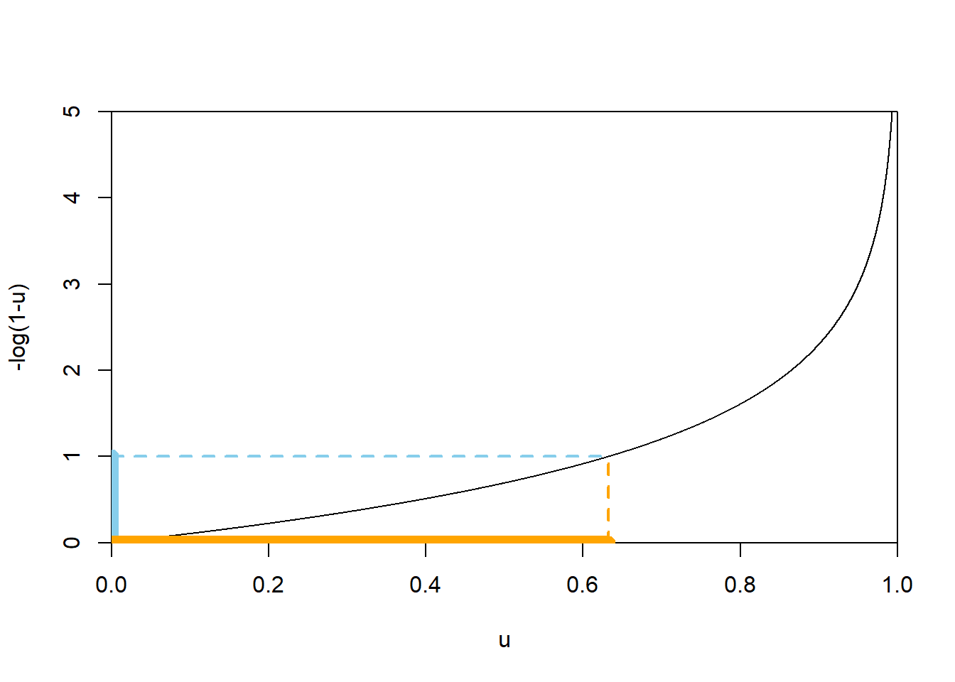
Figure 4.9: A plot of the function $u\mapsto -\log(1-u)$. The dotted lines illustrate that $-\log(1-u)\le 1$ if and only if $u\le 1-e^{-1}\approx 0.632$.

If $X$ is a continuous random variable whose distribution is known, the cdf method can be used to find the pdf of $Y=g(X)$

• Determine the possible values of $Y$. Let $y$ represent a generic possible value of $Y$.
• The cdf of $Y$ is $F_Y(y) = \textrm{P}(Y\le y) = \textrm{P}(g(X) \le y)$.
• Rearrange $\{g(X) \le y\}$ to get an event involving $X$. Warning: it is not always $\{X \le g^{-1}(y)\}$. Sketching a picture of the function $g$ helps.
• Obtain an expression for the cdf of $Y$ which involves $F_X$ and some transformation of the value $y$.
• Differentiate the expression for $F_Y(y)$ with respect to $y$, and use what is known about $F'_X = f_X$, to obtain the pdf of $Y$. You will typically need to apply the chain rule when differentiating.

You will need to use information about $X$ at some point in the last step above. You can either:

• Plug in the cdf of $X$ and then differentiate with respect to $y$.
• Differentiate with respect to $y$ and then plug in the pdf of $X$.

Either way gets you to the correct answer, but depending on the problem one way might be easier than the other. We’ll illustrate both methods in the next example.

Example 4.23 Let $X$ be a random variable with a Uniform(-1, 1) distribution and Let $Y=X^2$.

1. Sketch the pdf of $Y$.
2. Run a simulation to approximate the pdf of $Y$.
3. Find $F_Y(0.49)$.
4. Use the cdf method to find the pdf of $Y$. Is the pdf consistent with your simulation results?

Solution. to Example 4.23

Show/hide solution

1. First the possible values: since $-1< X<1$ we have $0<Y<1$. The idea to the sketch is that squaring a number less than 1 in absolute value returns a smaller number. So the transformation “pushes values towards 0” making the density higher near 0. Consider the intervals $[0, 0.1]$ and $[0.9, 1]$ on the original scale; both intervals have probability 0.05 under the Uniform($-1, 1$) distribution. On the squared scale, these intervals correspond to $[0, 0.01]$ and $[0.81, 1]$ respectively. So the 0.05 probability is “squished” into $[0, 0.01]$, resulting in a greater height, while it is “spread out” over $[0.81, 1]$ resulting in a smaller height. Remember: probability is represented by area.

2. See the simulation results below. We see that the density is highest near 0 and lowest near 1.

3. Since $X$ can take negative values, we have to be careful; see Figure 4.10 below. $$\{Y \le 0.49\} = \{X^2 \le 0.49\} = \{-\sqrt{0.49} \le X \le \sqrt{0.49}\}$$ Therefore, since $X$ has a Uniform($-1,1$) distribution, $$F_Y(0.49) = \textrm{P}(Y \le 0.49) = \textrm{P}(-0.7 \le X \le 0.7) = \frac{1.4}{2} = 0.7$$

4. Fix $0<y<1$. We now do the same calculation in the previous part in terms of a generic $y$, but it often helps to think of $y$ as a particular number first. $$\begin{align*} F_Y(y) & = \textrm{P}(Y\le y)\\ & = \textrm{P}(X^2\le y)\\ & = \textrm{P}(-\sqrt{y}\le X\le \sqrt{y})\\ & = F_X(\sqrt{y}) - F_X(-\sqrt{y}) \end{align*}$$ Note that the event of interest is not just $\{X\le \sqrt{y}\}$; see Figure 4.10 below. From here we can either

   use the cdf of $X$ and then differentiate, or differentiate and then use the pdf of $X$. We’ll illustrate both.

   1. Using the Uniform(-1, 1) cdf, the interval $[-\sqrt{y}, \sqrt{y}]$ has length $2\sqrt{y}$, and the total length of $[-1, 1]$ is 2, so we have $$F_Y(y) = F_X(\sqrt{y}) - F_X(-\sqrt{y}) = \frac{2\sqrt{y}}{2} = \sqrt{y}$$ Now differentiate with respect to the argument $y$ to obtain $f_Y(y) = \frac{1}{2\sqrt{y}}, 0<y<1$.
   2. Differentiate both sides of $F_Y(y) = F_X(\sqrt{y}) - F_X(-\sqrt{y})$, with respect to $y$. Differentiating the cdf $F_Y$ yields its pdf $f_Y$, and differentiating the cdf $F_X$ yields its pdf $f_X$. But don’t forget to use the chain rule when differentiating $F_X(\sqrt{y})$. $$\begin{align*} F_Y(y) & = F_X(\sqrt{y}) - F_X(-\sqrt{y})\\ \Rightarrow \frac{d}{dy} F_Y(y) & = \frac{d}{dy}\left(F_X(\sqrt{y}) - F_X(-\sqrt{y})\right)\\ \qquad f_Y(y) & = f_X(\sqrt{y})\frac{1}{2\sqrt{y}} - f_X(-\sqrt{y})\left(-\frac{1}{2\sqrt{y}}\right)\\ &= \frac{1}{2\sqrt{y}}\left(f_X(\sqrt{y})+f_X(-\sqrt{y})\right) \end{align*}$$ Since $X$ has a Uniform(-1, 1) distribution, its pdf is $f_X(x) = 1/2, -1<x<1$. But for $0<y<1$, $\sqrt{y}$ and $-\sqrt{y}$ are just numbers in $[-1, 1]$, so $f_X(\sqrt{y})=1/2$ and $f_X(-\sqrt{y})=1/2$. Therefore, $f_Y(y) = \frac{1}{2\sqrt{y}}, 0<y<1$. The histogram of simulated values seems consistent with this shape. (The density blows up at 0.)

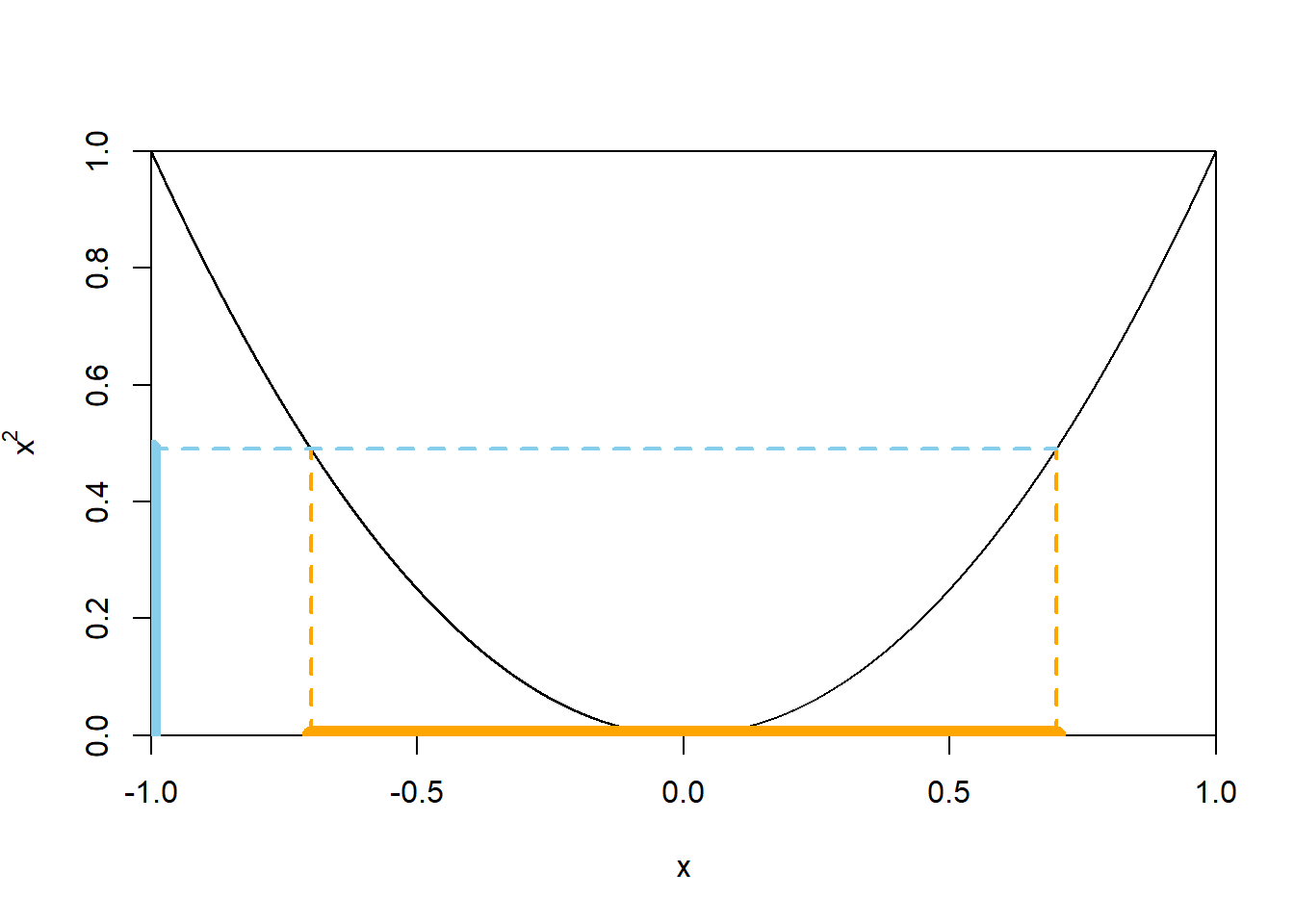
Figure 4.10: A plot of the function $x\mapsto x^2$ for $-1<x<1$. The dotted lines illustrate that $x^2\le 0.49$ if and only if $-\sqrt{0.49}\le x\le \sqrt{0.49}$.

X = RV(Uniform(-1, 1))
Y = X ** 2

Y.sim(10000).plot()

# plot the density
from numpy import *
y = linspace(0.001, 1, 1000)
plt.plot(y, 0.5 / sqrt(y), 'k-');
plt.ylim(0, 10);

plt.show()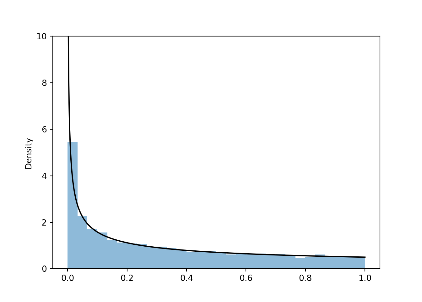

4.5.1 Transformations of multiple random variables

Cumulative distribution functions can also be used to derive the joint pdf of multiple random variables. If $F_{X, Y}$ is the joint cdf of $X$ and $Y$ then the joint pdf of $X$ and $Y$ is

$$f_{X, Y}(x, y) = \frac{\partial^2}{\partial x\partial y} F_{X, Y}(x, y)$$

Remember: when taking a partial derivative with respect to one variable, treat the other variables like constants.

Example 4.24 Recall the example in Section 3.8.3. Let $\textrm{P}$ be the probability space corresponding to two spins of the Uniform(1, 4) spinner, and let $X$ be the sum of the two spins, and $Y$ the larger spin (or the common value if a tie).

Solution. to Example 4.24

1. Let $F_{X, Y}$ denote the joint cdf of $X$ and $Y$. Find $F_{X, Y}(3.5, 2)$.
2. Find the joint cdf $F_{X, Y}$.
3. Find the joint pdf $f_{X, Y}$.

Show/hide solution

1. $F_{X, Y}(3.5, 2) = \textrm{P}(X \le 3.5, Y \le 2)$. The $(U_1, U_2)$ pairs take values in the square $[1, 4]\times[1, 4]$. Figure 4.11 illustrates the event $\{X \le 3.5, Y \le 2\}$. The shaded region has area $(1)(1)-(1/2)(0.5)(0.5) = 0.875$. Since $(U_1, U_2)$ pairs are uniformly distributed over the square region with area 9, $\textrm{P}(X \le 3.5, Y \le 2) = 3.875 / 9 = 0.0972$.
2. $F_{X, Y}(x, y) = \textrm{P}(X \le x, Y \le y)$. We repeat the calculation from the previous part with a generic $(x, y)$. Let $(x, y)$ be a possible value of $(X, Y)$; that is, $2<x<8$, $1<y<4$, and $y + 1 < x < 2y$. The event $\{X \le x, Y \le y\}$ will have a shape like the one in Figure 4.11, with area $(y-1)^2-(1/2)(2y-x)^2$. Since $(U_1, U_2)$ pairs are uniformly distributed over the square region with area 9 $$F_{X, Y}(x, y) = (1/9)\left((y-1)^2-(1/2)(2y-x)^2\right), \quad 2 < x < 8, 1 < y < 4, y + 1< x < 2y.$$
3. Differentiate the cdf with respect to both $x$ and $y$ $$\begin{align*} F_{X, Y}(x, y) & = (1/9)\left((y-1)^2-(1/2)(2y-x)^2\right)\\ \Rightarrow \frac{\partial}{\partial x}F_{X, Y}(x, y) & = \frac{\partial}{\partial x}(1/9)\left((y-1)^2-(1/2)(2y-x)^2\right)\\ & = (1/9)(2y-x)\\ \Rightarrow \frac{\partial^2}{\partial x\partial y}F_{X, Y}(x, y) & = \frac{\partial}{\partial y}(1/9)(2y-x)\\ = 2/9 \end{align*}$$ Therefore $$f_{X, Y}(x, y) = \begin{cases} 2/9, & 2<x<8,\; 1<y<4,\; x/2<y<x-1,\\ 0, & \text{otherwise} \end{cases}$$

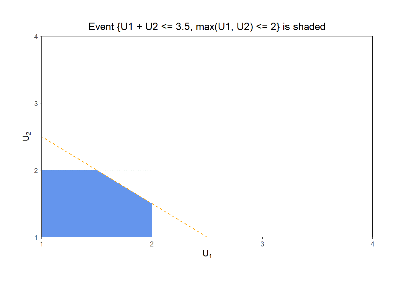
Figure 4.11: The event $\{X \le 3.2, Y \le 2\}$ for $X=U_1+U_2$, the sum, and $Y=\max(U_1, U_2)$, the max, of two spins $U_1, U_2$ of a Uniform(1, 4) spinner.

Example 4.25 Continuing Example 2.40, let $R$ be the random variable representing Regina’s arrival time in $[0, 1]$, and $Y$ for Cady. The random variable $T=\min(R, Y)$ represents the time in $(0, 1)$ at which the first person arrives. The random variable $W = |R - Y|$ represents the amount of time the first person to arrive waits for the second person to arrive.

1. Let $F_W$ be the cdf of $W$. Find $F_{W}(0.25)$.
2. Find the cdf $F_W$.
3. Find the pdf of $W$. What does this tell you about the distribution of waiting times?
4. Let $F_T$ be the cdf of $T$. Find $F_{T}(0.25)$.
5. Find the cdf $F_T$.
6. Find the pdf of $T$. What does this tell you about the time of the first arrival?
7. Are $T$ and $W$ the same random variable?
8. Do $T$ and $W$ have the same distribution?

Solution. to Example 4.25

Show/hide solution

1. $F_W(0.25) = \textrm{P}(W \le 0.25)$. We computed this in Example 2.40; $F_W(0.25) = 1 - (1-0.25)^2$. See the plot on the left in Figure 4.12 below.
2. We repeat the calculation in the previous part for a generic $w$ in $(0, 1)$. $$F_W(w) = 1 - (1 - w)^2, \quad 0 < w <1$$
3. Differentiate the cdf with respect to $w$. $$f_W(w) = 2(1 - w), \quad 0 < w <1$$ Waiting time has highest density for short waiting times and lowest density for long waiting times.
4. $F_T(0.25) = \textrm{P}(T \le 0.25)$. See the plot on the right in Figure 4.12 below. $\textrm{P}(T \le 0.25) = 1 - (1-0.25)^2$.
5. We repeat the calculation in the previous part for a generic $t$ in $(0, 1)$. $$F_T(t) = 1 - (1 - t)^2, \quad 0 < t <1$$
6. Differentiate the pdf with respect to $t$. $$f_T(t) = 2(1 - t), \quad 0 < t <1$$ Time of first arrival has highest density near 0 and lowest density near 1.
7. No, $T$ and $W$ are not the same random variable. For example, if they both arrive at time 0.5, then $T$ is 0.5 but $W$ is 0.
8. Yes, they do have the same distribution. They have the same pdf (and cdf).

Figure 4.12: Illustration of the events $\{W \le 0.25\}$ in Example 4.25. The square represents the sample space $\Omega=[0,1]\times[0,1]$.

R, Y = RV(Uniform(0, 1) ** 2)

W = abs(R - Y)

T = (R & Y).apply(min)

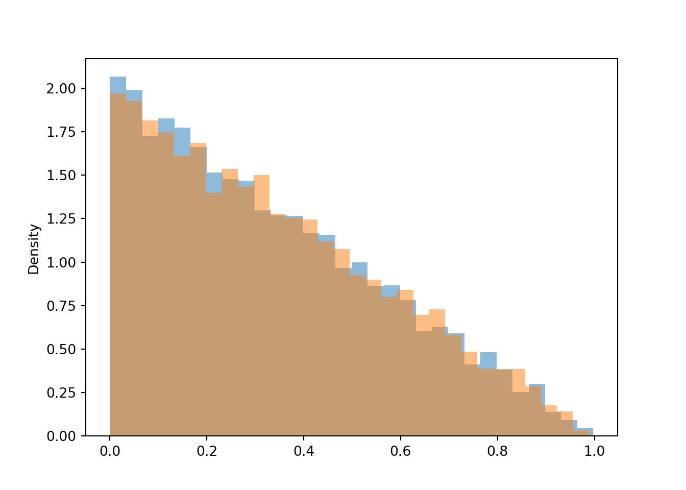
W.sim(10000).plot()
T.sim(10000).plot()
plt.show()