Chapter 22: R
22.1 TonyKuoYJ
郭耀仁 認識 R 的美好
https://bookdown.org/tonykuoyj/eloquentr/getting-started.html
https://bookdown.org/tonykuoyj/eloquentr/easy-installation.html#about-packages
install.pacakges()
library()
https://bookdown.org/tonykuoyj/eloquentr/getting-started.html
22.1.1 quick intro
Ctrl + Alt + I to insert a new code chunk in RStudio
Ctrl + Enter to run the current line
Ctrl + Shift + Enter to run the current chunk
##                _
## platform       x86_64-w64-mingw32
## arch           x86_64
## os             mingw32
## crt            ucrt
## system         x86_64, mingw32
## status
## major          4
## minor          2.1
## year           2022
## month          06
## day            23
## svn rev        82513
## language       R
## version.string R version 4.2.1 (2022-06-23 ucrt)
## nickname Funny-Looking Kid## [1] 23## [1] 11 13Ctrl + L to clean R console
path with slash / in R, differing backslash \ in M$ Windows
22.1.2 R style
https://bookdown.org/tonykuoyj/eloquentr/styleguide.html
snake_case rather than camelCase
22.1.3 data workflow or forward pipe
from chaining method in object-oriented programming to functional programming
22.1.3.1 %>% operator
## [1] 5 4 3 2 1 0 1 2 3 4 5##
## Attaching package: 'magrittr'## The following object is masked _by_ '.GlobalEnv':
##
## add## [1] 5 4 3 2 1 0 1 2 3 4 5# with readability but too many lines
sys_date <- Sys.Date()
sys_date_yr <- format(sys_date, format = "%Y")
sys_date_num <- as.numeric(sys_date_yr)
sys_date_num## [1] 2025# less line but also less readability
sys_date_num <- as.numeric(format(Sys.Date(), format = "%Y"))
sys_date_num## [1] 2025# use %>% operator to demonstrate data workflow or forward pipe
sys_date_num <- Sys.Date() %>%
format(format = "%Y") %>%
as.numeric()
sys_date_num## [1] 202522.1.4 data processing with dplyr
https://bookdown.org/tonykuoyj/eloquentr/dplyr.html
some functions functioning like those in SQL
## Warning: package 'dplyr' was built under R version 4.2.3##
## Attaching package: 'dplyr'## The following objects are masked from 'package:stats':
##
## filter, lag## The following objects are masked from 'package:base':
##
## intersect, setdiff, setequal, union## Warning: package 'gapminder' was built under R version 4.2.3## # A tibble: 6 × 6
## country continent year lifeExp pop gdpPercap
## <fct> <fct> <int> <dbl> <int> <dbl>
## 1 Afghanistan Asia 1952 28.8 8425333 779.
## 2 Afghanistan Asia 1957 30.3 9240934 821.
## 3 Afghanistan Asia 1962 32.0 10267083 853.
## 4 Afghanistan Asia 1967 34.0 11537966 836.
## 5 Afghanistan Asia 1972 36.1 13079460 740.
## 6 Afghanistan Asia 1977 38.4 14880372 786.## # A tibble: 142 × 6
## country continent year lifeExp pop gdpPercap
## <fct> <fct> <int> <dbl> <int> <dbl>
## 1 Afghanistan Asia 2007 43.8 31889923 975.
## 2 Albania Europe 2007 76.4 3600523 5937.
## 3 Algeria Africa 2007 72.3 33333216 6223.
## 4 Angola Africa 2007 42.7 12420476 4797.
## 5 Argentina Americas 2007 75.3 40301927 12779.
## 6 Australia Oceania 2007 81.2 20434176 34435.
## 7 Austria Europe 2007 79.8 8199783 36126.
## 8 Bahrain Asia 2007 75.6 708573 29796.
## 9 Bangladesh Asia 2007 64.1 150448339 1391.
## 10 Belgium Europe 2007 79.4 10392226 33693.
## # ℹ 132 more rowslibrary(gapminder)
library(dplyr)
library(magrittr)
gapminder %>%
filter(year == 2007) %>%
select(country)## # A tibble: 142 × 1
## country
## <fct>
## 1 Afghanistan
## 2 Albania
## 3 Algeria
## 4 Angola
## 5 Argentina
## 6 Australia
## 7 Austria
## 8 Bahrain
## 9 Bangladesh
## 10 Belgium
## # ℹ 132 more rowslibrary(gapminder)
library(dplyr)
library(magrittr)
gapminder %>%
mutate(pop_in_thousands = pop / 1000)## # A tibble: 1,704 × 7
## country continent year lifeExp pop gdpPercap pop_in_thousands
## <fct> <fct> <int> <dbl> <int> <dbl> <dbl>
## 1 Afghanistan Asia 1952 28.8 8425333 779. 8425.
## 2 Afghanistan Asia 1957 30.3 9240934 821. 9241.
## 3 Afghanistan Asia 1962 32.0 10267083 853. 10267.
## 4 Afghanistan Asia 1967 34.0 11537966 836. 11538.
## 5 Afghanistan Asia 1972 36.1 13079460 740. 13079.
## 6 Afghanistan Asia 1977 38.4 14880372 786. 14880.
## 7 Afghanistan Asia 1982 39.9 12881816 978. 12882.
## 8 Afghanistan Asia 1987 40.8 13867957 852. 13868.
## 9 Afghanistan Asia 1992 41.7 16317921 649. 16318.
## 10 Afghanistan Asia 1997 41.8 22227415 635. 22227.
## # ℹ 1,694 more rows## # A tibble: 1,704 × 6
## country continent year lifeExp pop gdpPercap
## <fct> <fct> <int> <dbl> <int> <dbl>
## 1 Afghanistan Asia 1952 28.8 8425333 779.
## 2 Albania Europe 1952 55.2 1282697 1601.
## 3 Algeria Africa 1952 43.1 9279525 2449.
## 4 Angola Africa 1952 30.0 4232095 3521.
## 5 Argentina Americas 1952 62.5 17876956 5911.
## 6 Australia Oceania 1952 69.1 8691212 10040.
## 7 Austria Europe 1952 66.8 6927772 6137.
## 8 Bahrain Asia 1952 50.9 120447 9867.
## 9 Bangladesh Asia 1952 37.5 46886859 684.
## 10 Belgium Europe 1952 68 8730405 8343.
## # ℹ 1,694 more rowstotal population in the world in 2007
library(gapminder)
library(dplyr)
library(magrittr)

gapminder %>%
filter(year == 2007) %>%
summarise(ttl_pop = sum(as.numeric(pop)))## # A tibble: 1 × 1
## ttl_pop
## <dbl>
## 1 6251013179total population group by the continents in 2007
library(gapminder)
library(dplyr)
library(magrittr)

gapminder %>%
  filter(year == 2007) %>%
  group_by(continent) %>%
  summarise(ttl_pop = sum(as.numeric(pop)))
## # A tibble: 5 × 2
## continent ttl_pop
## <fct> <dbl>
## 1 Africa 929539692
## 2 Americas 898871184
## 3 Asia 3811953827
## 4 Europe 586098529
## 5 Oceania 2454994722.1.5 visualization statically with ggplot2
## Warning: package 'ggplot2' was built under R version 4.2.3library(gapminder)
gapminder_2007 <- gapminder %>%
filter(year == 2007)
scatter_plot <- ggplot(gapminder_2007, aes(x = gdpPercap, y = lifeExp)) +
geom_point()
scatter_plot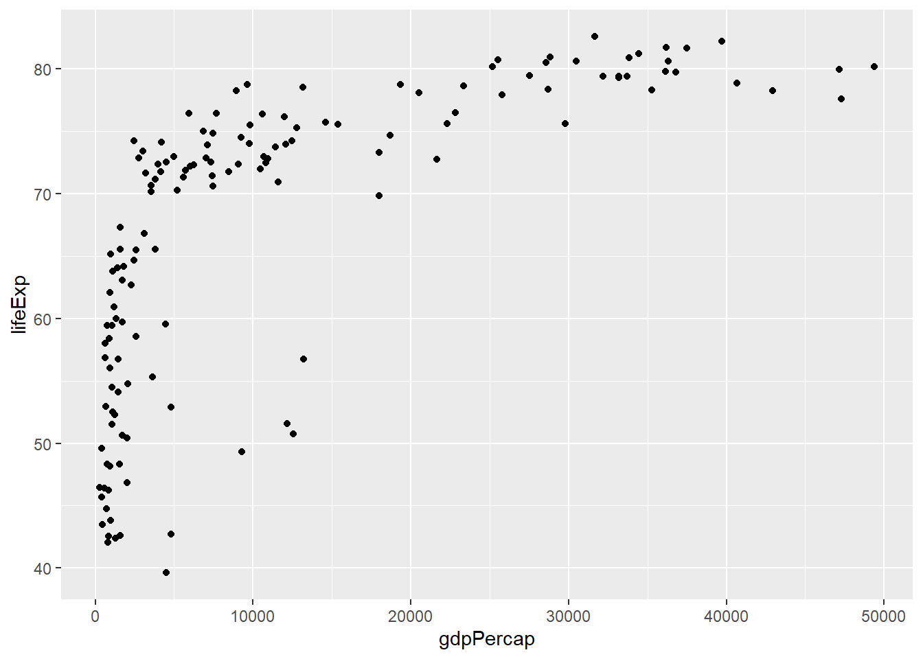
library(ggplot2)
library(gapminder)

north_asia <- gapminder %>%
  filter(country %in% c("China", "Japan", "Taiwan", "Korea, Rep."))
line_plot <- ggplot(north_asia, aes(x = year, y = gdpPercap, colour = country)) +
  geom_line()
line_plot
library(ggplot2)
library(gapminder)

hist_plot <- ggplot(gapminder_2007, aes(x = gdpPercap)) +
  geom_histogram()
hist_plot
## `stat_bin()` using `bins = 30`. Pick better value with `binwidth`.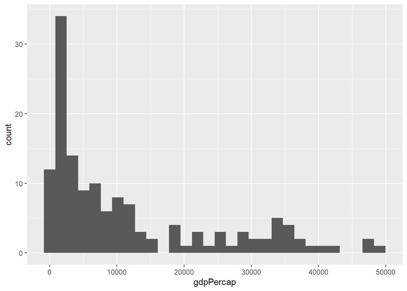

library(ggplot2)
library(gapminder)

box_plot <- ggplot(gapminder_2007, aes(x = continent, y = gdpPercap)) +
  geom_boxplot()
box_plot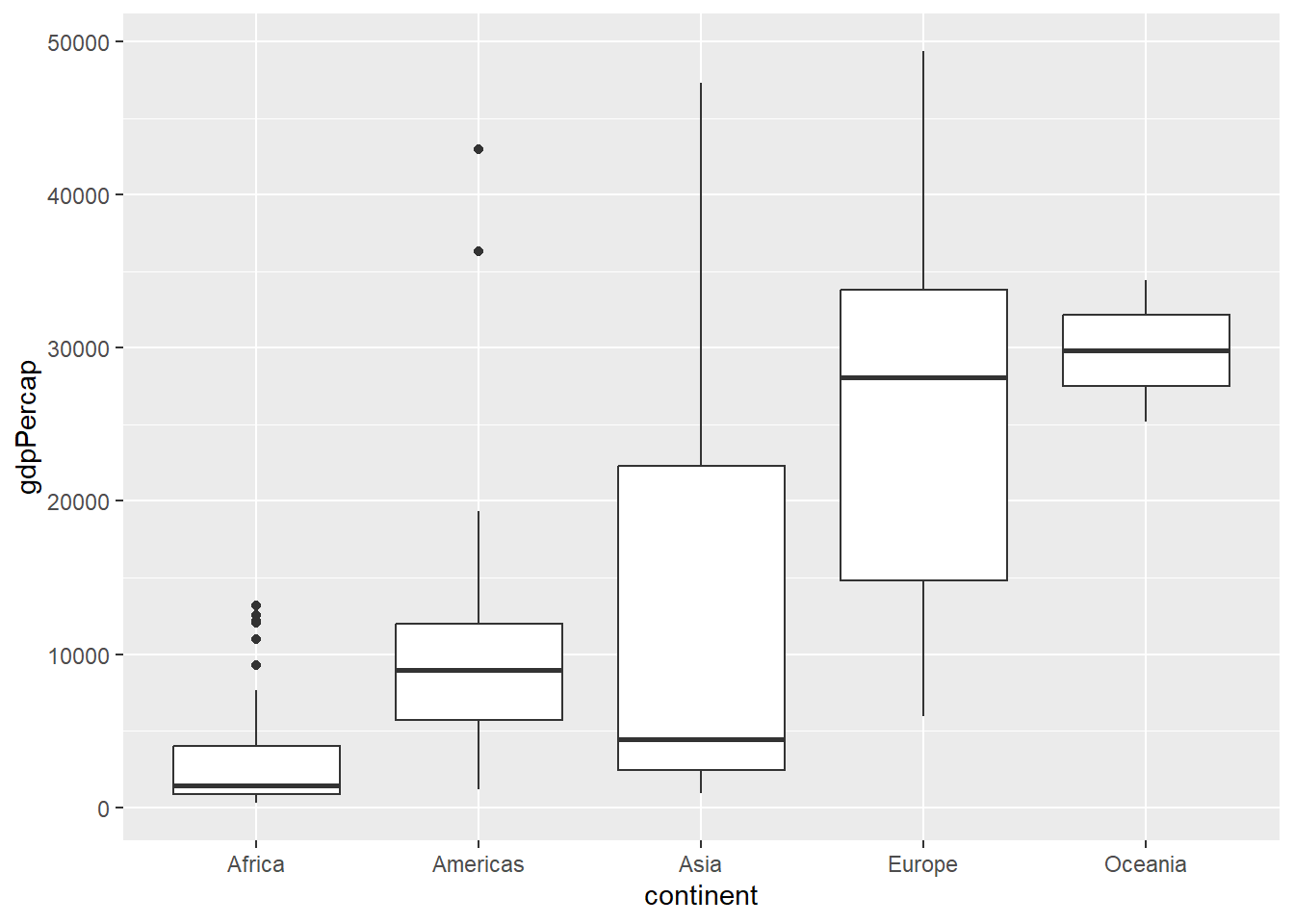
library(ggplot2)
library(gapminder)

gdpPercap_2007_na <- gapminder %>%
  filter(year == 2007 & country %in% c("China", "Japan", "Taiwan", "Korea, Rep."))
bar_plot <- ggplot(gdpPercap_2007_na, aes(x = country, y = gdpPercap)) +
  geom_bar(stat = "identity")
bar_plot
22.1.6 loop
https://bookdown.org/tonykuoyj/eloquentr/for.html
##  [1] "January"   "February"  "March"     "April"     "May"       "June"
## [7] "July" "August" "September" "October" "November" "December"## [1] "January"## [1] "January"
## [1] "February"
## [1] "March"
## [1] "April"
## [1] "May"
## [1] "June"
## [1] "July"
## [1] "August"
## [1] "September"
## [1] "October"
## [1] "November"
## [1] "December"22.1.7 variable type
https://bookdown.org/tonykuoyj/eloquentr/variable-types.html
https://www.w3schools.com/r/r_data_types.asp
- numeric
- integer
- complex = complex number
- character
- logical = boolean
## [1] "integer"## [1] "integer"## [1] "numeric"time: POSIXct POSIXt
## [1] "POSIXct" "POSIXt"## [1] TRUE22.1.7.1 date
1970-01-01 = 0L
## [1] 0check if type of x is Date
inherits(x, what = "Date")
convert character to Date
as.Date("01-01-1970", format = "%m-%d-%Y")
22.1.8 data type
https://bookdown.org/tonykuoyj/eloquentr/vector-factor.html
- 1D
- 2D
- \(n\)D
22.1.8.1 vector
## [1] "spring" "summer" "autumn" "winter"## [1] "autumn"## [1] "spring" "autumn"only one variable type for a vector
## [1] "numeric"## [1] 7 0## [1] "integer"## [1] "TRUE" "7" "24" "spring"## [1] "character"## [1] "character"## [1] "character"22.1.8.1.1 logic
four_seasons <- c("spring", "summer", "autumn", "winter")
my_favorite_seasons <- four_seasons == "spring" | four_seasons == "autumn"
four_seasons[my_favorite_seasons]
## [1] "spring" "autumn"22.1.8.2 factor
https://bookdown.org/tonykuoyj/eloquentr/vector-factor.html#factor
## [1] "spring" "summer" "autumn" "winter"## [1] spring summer autumn winter
## Levels: autumn spring summer winterfour_seasons <- c("spring", "summer", "autumn", "winter")
four_seasons_factor <- factor(four_seasons, ordered = TRUE, levels = c("summer", "winter", "spring", "autumn"))
four_seasons_factor## [1] spring summer autumn winter
## Levels: summer < winter < spring < autumntemperatures <- c("warm", "hot", "cold")
temp_factors <- factor(temperatures, ordered = TRUE, levels = c("cold", "warm", "hot"))
temp_factors## [1] warm hot cold
## Levels: cold < warm < hotif no levels specified, the levels will be specified alphabetically, sometimes not really true
temperatures <- c("warm", "hot", "cold")
temp_factors <- factor(temperatures, ordered = TRUE)
temp_factors
## [1] warm hot cold
## Levels: cold < hot < warm22.1.8.3 matrix
https://bookdown.org/tonykuoyj/eloquentr/matrix-dataframe-more.html
##      [,1] [,2] [,3]
## [1,]    1    3    5
## [2,] 2 4 6## [1] "matrix" "array"## [,1] [,2] [,3]
## [1,] 1 2 3
## [2,] 4 5 6## [1] 6## [1] 4 5 6## [1] 3 6## [1] 4 2 5 3boolean will become value in a matrix, like vector
##      [,1] [,2] [,3]
## [1,]    1    1    3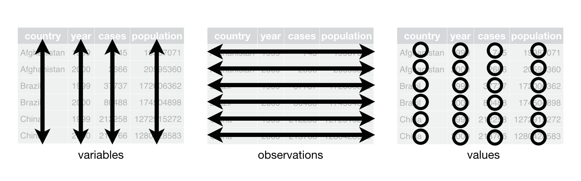
## [2,] 2 0 4## [1] "numeric"22.1.8.4 data frame
- variable: column
- observation: row
- value: cell
team_name <- c("Chicago Bulls", "Golden State Warriors")
wins <- c(72, 73)
losses <- c(10, 9)
is_champion <- c(TRUE, FALSE)
season <- c("1995-96", "2015-16")

great_nba_teams <- data.frame(team_name, wins, losses, is_champion, season)
great_nba_teams
## team_name wins losses is_champion season
## 1 Chicago Bulls 72 10 TRUE 1995-96
## 2 Golden State Warriors 73 9 FALSE 2015-16## [1] "Chicago Bulls"## team_name wins losses is_champion season
## 1 Chicago Bulls 72 10 TRUE 1995-96## [1] "Chicago Bulls" "Golden State Warriors"stringsAsFactors = TRUE
team_name <- c("Chicago Bulls", "Golden State Warriors")
wins <- c(72, 73)
losses <- c(10, 9)
is_champion <- c(TRUE, FALSE)
season <- c("1995-96", "2015-16")

great_nba_teams <- data.frame(team_name, wins, losses, is_champion, season, stringsAsFactors = TRUE)
great_nba_teams[, 1]
## [1] Chicago Bulls Golden State Warriors
## Levels: Chicago Bulls Golden State WarriorsstringsAsFactors = FALSE
team_name <- c("Chicago Bulls", "Golden State Warriors")
wins <- c(72, 73)
losses <- c(10, 9)
is_champion <- c(TRUE, FALSE)
season <- c("1995-96", "2015-16")

great_nba_teams <- data.frame(team_name, wins, losses, is_champion, season, stringsAsFactors = FALSE)
great_nba_teams[, 1]
## [1] "Chicago Bulls" "Golden State Warriors"22.1.8.4.1 selecting variable or column
## [1] "Chicago Bulls" "Golden State Warriors"## [1] "Chicago Bulls" "Golden State Warriors"22.2 W3School
https://www.w3schools.com/r/default.asp
22.2.1 same multiple variable
https://www.w3schools.com/r/r_variables_multiple.asp
# Assign the same value to multiple variables in one line
var1 <- var2 <- var3 <- "Orange"

# Print variable values
var1
## [1] "Orange"## [1] "Orange"## [1] "Orange"22.2.3 complex number
22.2.5 global assignment <<-
## [1] "R is fantastic"## [1] "fantastic"## [1] "R is fantastic"## [1] "R is fantastic"22.2.6 data type
22.2.6.1 array
https://www.w3schools.com/r/r_arrays.asp
## [1] 1 2 3 4 5 6 7 8 9 10 11 12 13 14 15 16 17 18 19 20 21 22 23 24## , , 1
##
## [,1] [,2] [,3]
## [1,] 1 5 9
## [2,] 2 6 10
## [3,] 3 7 11
## [4,] 4 8 12
##
## , , 2
##
## [,1] [,2] [,3]
## [1,] 13 17 21
## [2,] 14 18 22
## [3,] 15 19 23
## [4,] 16 20 24## [1] 2222.3 Apan Liao
R 演習室
https://www.youtube.com/playlist?list=PL5AC0ADBF65924EAD
22.3.1 data input
https://www.youtube.com/watch?v=STcIxf_vUWY&list=PL5AC0ADBF65924EAD&index=1
scan()- read
read.table()read.csv()
22.3.2 descriptive statistics
https://www.youtube.com/watch?v=GL3Wv_45LaU&list=PL5AC0ADBF65924EAD&index=2