Chapter 16: TikZ

Ti$k$Z
- PGFplots^[16.5]
- tikzplotlib^[16.6]: Python^[15] matplotlib^[30] export to TikZ^[16] .tex

multi-column 10.3.6

knitr::opts_chunk$set(fig.pos = "H", out.extra = "")

https://bookdown.org/yihui/rmarkdown-cookbook/html-scroll.html

\begin{tikzpicture}
  \draw (-1,1)--(0,0)--(1,2);
\end{tikzpicture}

How to speed up bookdown generation?

https://stackoverflow.com/questions/56541371/how-to-speed-up-bookdown-generation

TikZ and PGFplots

What’s the relation between packages PGFplots and TikZ?

https://tex.stackexchange.com/questions/285925/whats-the-relation-between-packages-pgfplots-and-tikz

https://www.youtube.com/watch?v=bQugbYq0BVA

https://www.youtube.com/watch?v=ft4Kg9emK1k&list=PLg5nrpKdkk2DWcg3scb75AknF7DJXs8lk&index=18

\begin{tikzpicture}
  \def\a{1.5} % amplitude
  \def\b{2}   % frequency
  \draw[->] (-0.2,0)--(4.2,0) node[right, font=\small] {$x$};
  \draw[->] (0,-4)--(0,0.5) node[above] {$y$};
  \draw[domain=0:4,smooth,variable=\t,blue,thick] 
    plot ({\a * (\b*\t - sin(deg(\b*\t)))},{-\a * (1 - cos(deg(\b*\t)))});
  % \node[above] at (2, 0.5) {Brachistochrone Curve};
  \node[above, font=\footnotesize] at (2, 1) {Brachistochrone Curve};
  \node[above, font=\footnotesize] at (2, 0) {$\begin{aligned}
& x=r(t-\sin t) \\
& y=r(1-\cos t)
\end{aligned}$};
\end{tikzpicture}

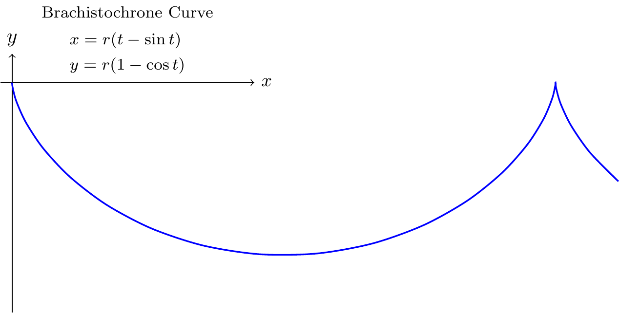
Fig. 16.1: Brachistochrone Curve

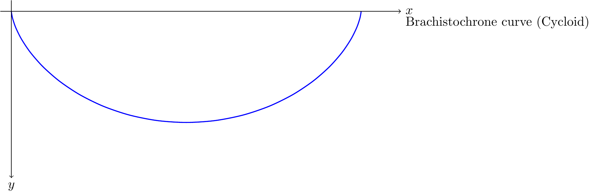
Fig. 16.2: Brachistochrone Curve

16.1 2D

https://zhuanlan.zhihu.com/p/127155579?utm_psn=1741479950987960320

\begin{tikzpicture}
  \draw (-1,1)--(0,0)--(1,2);
\end{tikzpicture}

\begin{tikzpicture}
  \draw (-1,1)--(0,0)--(1,2);
\end{tikzpicture}

out.width=if (knitr:::is_html_output()) '20%'

\begin{tikzpicture}
  \draw (-1,1)--(0,0)--(1,2);
\end{tikzpicture}

\begin{tikzpicture}
  \draw[rounded corners] (-1,1)--(0,0)--(1,2)--(-1,1);
\end{tikzpicture}

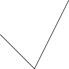
Fig. 16.3: rounded corner pseudo-closed triangle

\begin{tikzpicture}
  \draw[rounded corners] (-1,1)--(0,0)--(1,2)--cycle;
\end{tikzpicture}

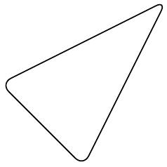
Fig. 16.4: rounded corner triangle

\begin{tikzpicture}
  \draw[rounded corners] (-1,1)--(0,0)--(1,2)--cycle;
  \draw[rounded corners] (-1,1)--(0,0)--(1,2)--(-1,1);
\end{tikzpicture}

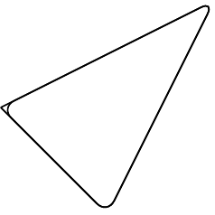
Fig. 16.5: triangle vs. pseudo-closed triangle

\begin{tikzpicture}
  \draw (0,0) rectangle (4,2);
\end{tikzpicture}

Fig. 16.6: rectangle

\begin{tikzpicture}
  \draw (0,0) rectangle (2,2);
\end{tikzpicture}

Fig. 16.7: square

\begin{tikzpicture}
  \draw (0,0) circle (1);
\end{tikzpicture}

Fig. 10.2: circle

\begin{tikzpicture}
  \draw (0,0) circle (1);
  \draw (0,0) rectangle (2,2);
\end{tikzpicture}

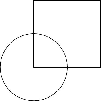
Fig. 10.3: circle and square

\begin{tikzpicture}
  \draw (1,1) ellipse (2 and 1);
\end{tikzpicture}

Fig. 16.8: ellipse

\begin{tikzpicture}
  \draw (1 ,1) arc (0:270:1);
  \draw (6 ,1) arc (0:270:2 and 1);
\end{tikzpicture}

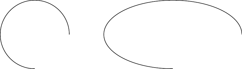
Fig. 16.9: circle and ellipse arcs

\begin{tikzpicture}
  \draw (-1,1) parabola bend (0,0) (2,4);
\end{tikzpicture}

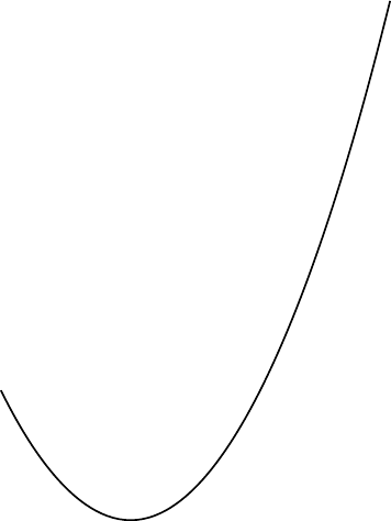
Fig. 16.10: parabola arc

\begin{tikzpicture}
  \draw (-1,1) parabola bend (0,0) (2,4);
  \filldraw
    (-1,1) circle (.05)
    ( 0,0) circle (.05)
    ( 1,1) circle (.05)
    ( 2,4) circle (.05);
\end{tikzpicture}

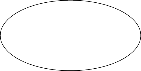
Fig. 16.11: parabola arc with points

\begin{tikzpicture}
  \draw[step=20pt] (0,0) grid (3,2);
  \draw[help lines ,step=20pt] (4,0) grid (7,2);
\end{tikzpicture}

Fig. 16.12: grid and help lines

\begin{tikzpicture}[scale=0.25]
  \draw[->] (0,0)--(9,0);
  \draw[<-] (0,1)--(9,1);
  \draw[<->] (0,2)--(9,2);
  \draw[>->>] (0,3)--(9,3);
  \draw[|<->|] (0,4)--(9,4);
\end{tikzpicture}

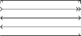
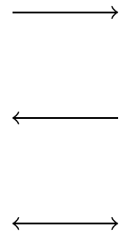
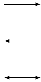
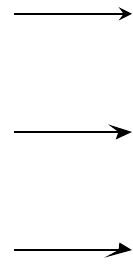
Fig. 16.13: arrows

\begin{tikzpicture}
  \draw[line width =2pt] (0,6)--(9,6); 
  \draw[dotted]          (0,5)--(9,5); 
  \draw[densely dotted]  (0,4)--(9,4); 
  \draw[loosely dotted]  (0,3)--(9,3); 
  \draw[dashed]          (0,2)--(9,2); 
  \draw[densely dashed]  (0,1)--(9,1); 
  \draw[loosely dashed]  (0,0)--(9,0);
\end{tikzpicture}

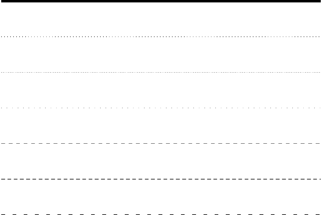
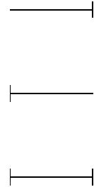
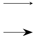
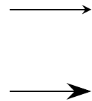
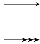
Fig. 16.14: lines

\begin{tikzpicture}[dline/.style={color= blue, line width=2pt}]
  \draw[dline] (0,0)--(9,0); 
\end{tikzpicture}

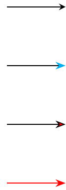
Fig. 16.15: head styling

\begin{tikzpicture}
  \draw (0,0) rectangle (2,2);
  \draw[shift={( 3, 0)}] (0,0) rectangle (2,2);
  \draw[shift={( 0, 3)}] (0,0) rectangle (2,2);
  \draw[shift={( 0,-3)}] (0,0) rectangle (2,2);
  \draw[shift={(-3, 0)}] (0,0) rectangle (2,2);
  \draw[shift={( 3, 3)}] (0,0) rectangle (2,2);
  \draw[shift={(-3, 3)}] (0,0) rectangle (2,2);
  \draw[shift={( 3,-3)}] (0,0) rectangle (2,2);
  \draw[shift={(-3,-3)}] (0,0) rectangle (2,2);
\end{tikzpicture}

Fig. 16.16: transform: shift

\begin{tikzpicture}
  \draw (0,0) rectangle (2,2);
  \draw[xshift= 100pt] (0,0) rectangle (2,2);
  \draw[xshift=-100pt] (0,0) rectangle (2,2);
  \draw[yshift= 100pt] (0,0) rectangle (2,2);
  \draw[yshift=-100pt] (0,0) rectangle (2,2);
\end{tikzpicture}

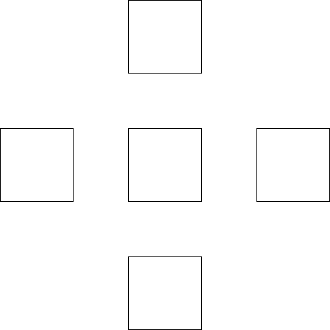
Fig. 16.17: transform: shift x, y

\begin{tikzpicture}
  \draw (0,0) rectangle (2,2);
  \draw[xshift= 100pt, xscale=1.5] (0,0) rectangle (2,2);
  \draw[yshift= 100pt, xscale=0.5] (0,0) rectangle (2,2);
  \draw[xshift=-100pt, yscale=1.5] (0,0) rectangle (2,2);
  \draw[yshift=-100pt, yscale=0.5] (0,0) rectangle (2,2);
\end{tikzpicture}

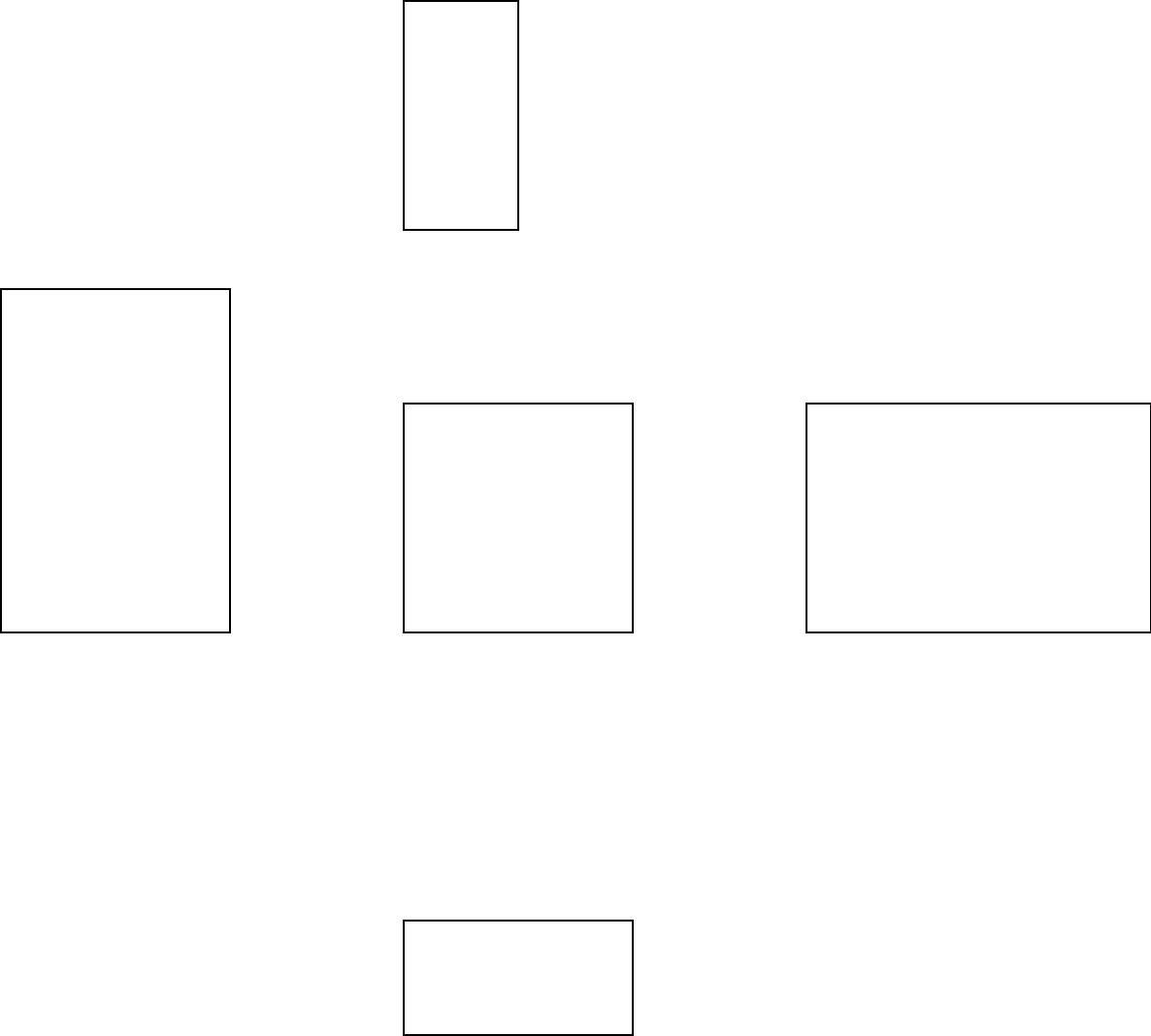
Fig. 16.18: transform: scale x, y

\begin{tikzpicture}
  \draw (0,0) rectangle (2,2);
  \draw[xshift= 100pt, xscale=1.5] (0,0) rectangle (2,2);
  \draw[yshift= 100pt, yscale=1.5] (0,0) rectangle (2,2);
  \draw[xshift=-100pt, xscale=0.5] (0,0) rectangle (2,2);
  \draw[yshift=-100pt, yscale=0.5] (0,0) rectangle (2,2);
\end{tikzpicture}

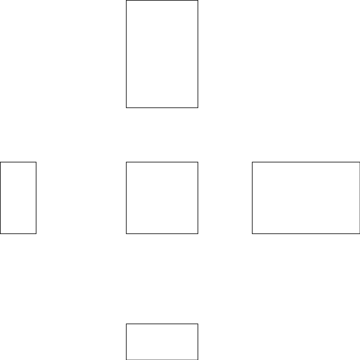
Fig. 16.19: transform: scale

\begin{tikzpicture}
  \draw (0,0) rectangle (2,2);
  \draw[xshift=125pt,rotate=45] (0,0) rectangle (2,2);
  \draw[xshift=175pt,rotate around={45:(2 ,2)}] (0,0) rectangle (2,2);
\end{tikzpicture}

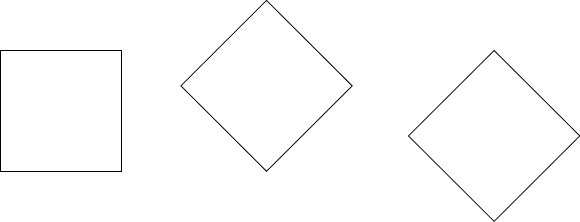
Fig. 16.20: transform: rotate

\begin{tikzpicture}
  \draw (0,0) rectangle (2,2);
  \draw[xshift=70pt,xslant=1] (0,0) rectangle (2,2);
  \draw[yshift=70pt,yslant=1] (0,0) rectangle (2,2);
\end{tikzpicture}

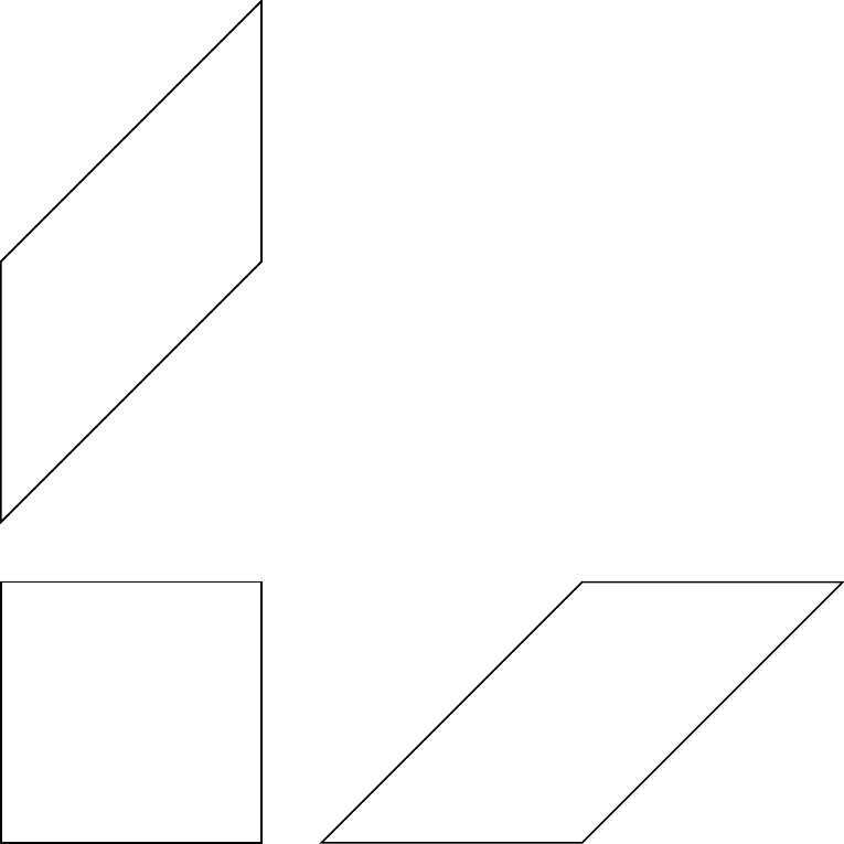
Fig. 16.21: transform: slant

\tikzset{
  box/.style={
    draw=blue,
    rectangle,
    rounded corners=5pt,
    minimum width=50pt,
    minimum height=20pt,
    inner sep=5pt
  }
}
\begin{tikzpicture}
  \node[box] (1) at (0,0) {1};
  \node[box] (2) at (4,0) {2};
  \node[box] (3) at (8,0) {3};
  \draw[->] (1)--(2);
  \draw[->] (2)--(3);
  \node at (2,1) {a};
  \node at (6,1) {b};
\end{tikzpicture}

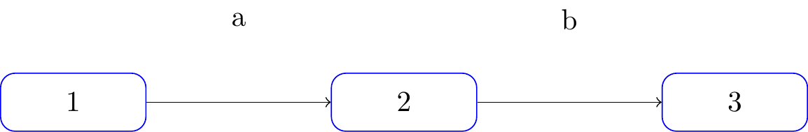
Fig. 16.22: flowchart

\tikzset{
  box/.style={
    draw=blue,
    fill=blue!20,
    rectangle,
    rounded corners=5pt,
    minimum height=20pt,
    inner sep=5pt
  }
}
\begin{tikzpicture}
  \node[box] {1}
      child {node[box] {2}}
      child {node[box] {3}
          child {node[box] {4}}
          child {node[box] {5}}
          child {node[box] {6}}
      };
\end{tikzpicture}

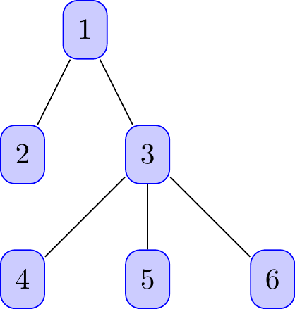
Fig. 16.23: tree

\begin{tikzpicture}
  \draw[->] (-0.2,0)--(6,0) node[right] {$x$};
  \draw[->] (0,-0.2)--(0,6) node[above] {$f(x)$};
  \draw[domain=0:4] plot (\x ,{0.1* exp(\x)}) node[right] {$f(x)=\frac{1}{10}e^x$};
\end{tikzpicture}

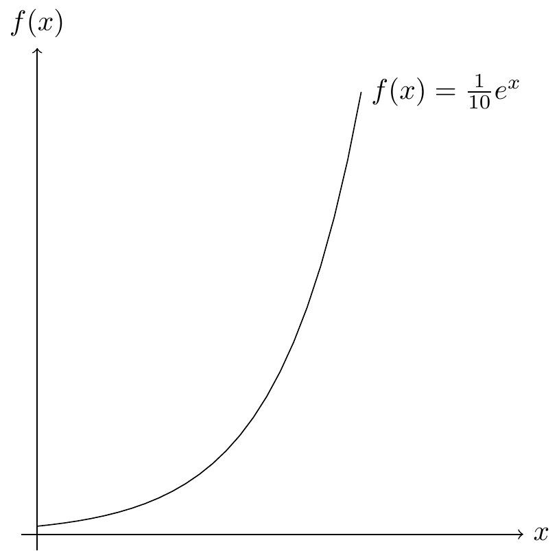
Fig. 16.24: function plot

https://stackoverflow.com/questions/64897575/tikz-libraries-in-bookdown

It turns out that you can simply put the \usetikzlibrary{...} command directly before the \begin{tikzpicture} and everything works fine :)

https://stackoverflow.com/questions/56211210/r-markdown-document-with-html-docx-output-using-latex-package-bbm

https://tex.stackexchange.com/questions/171711/how-to-include-latex-package-in-r-markdown

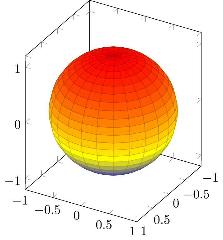
16.2 3D

https://zhuanlan.zhihu.com/p/431732330?utm_psn=1741857547550638080

https://github.com/RRWWW/Stereometry

\begin{tikzpicture}
  \coordinate (A) at ( 1, 1, 1);
  \coordinate (B) at ( 1, 1,-1);
  \coordinate (C) at ( 1,-1,-1);
  \coordinate (D) at ( 1,-1, 1);
  \coordinate (E) at (-1,-1, 1);
  \coordinate (F) at (-1,-1,-1);
  \coordinate (G) at (-1, 1,-1);
  \coordinate (H) at (-1, 1, 1);
  \draw (A) node[right=1pt] {$A$}--
        (B) node[right=1pt] {$B$}--
        (C) node[right=1pt] {$C$}--
        (D) node[right=1pt] {$D$}--
        (E) node[left= 1pt] {$E$}--
        (F) node[right=1pt] {$F$}--
        (G) node[right=1pt] {$G$}--
        (H) node[left= 1pt] {$H$}--
        (A) node[right=1pt] {$A$};
\end{tikzpicture}

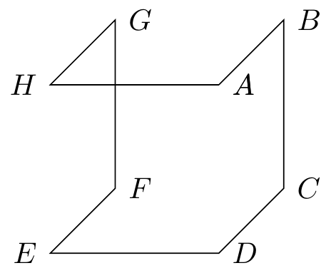
Fig. 16.25: cube

\usetikzlibrary{patterns}
\usetikzlibrary{3d,calc}
\tdplotsetmaincoords{45}{45}
\begin{tikzpicture}[tdplot_main_coords]
  \coordinate (A) at ( 1, 1, 1);
  \coordinate (B) at ( 1, 1,-1);
  \coordinate (C) at ( 1,-1,-1);
  \coordinate (D) at ( 1,-1, 1);
  \coordinate (E) at (-1,-1, 1);
  \coordinate (F) at (-1,-1,-1);
  \coordinate (G) at (-1, 1,-1);
  \coordinate (H) at (-1, 1, 1);
  \draw (A) node[right=1pt] {$A$}--
        (B) node[right=1pt] {$B$}--
        (C) node[right=1pt] {$C$}--
        (D) node[right=1pt] {$D$}--
        (E) node[left= 1pt] {$E$}--
        (F) node[right=1pt] {$F$}--
        (G) node[right=1pt] {$G$}--
        (H) node[left= 1pt] {$H$}--
        (A) node[right=1pt] {$A$};
\end{tikzpicture}

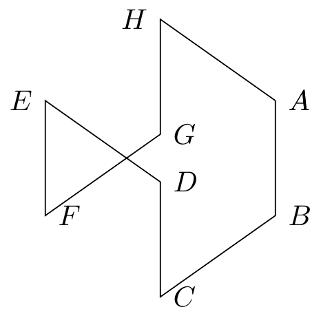
Fig. 16.26: cube rotate

\usetikzlibrary{patterns}
\usetikzlibrary{3d,calc}
%\tdplotsetmaincoords{70}{110}
\begin{tikzpicture}[rotate around y=-15, rotate around z=7]
  \coordinate (A) at ( 1, 1, 1);
  \coordinate (B) at ( 1, 1,-1);
  \coordinate (C) at ( 1,-1,-1);
  \coordinate (D) at ( 1,-1, 1);
  \coordinate (E) at (-1,-1, 1);
  \coordinate (F) at (-1,-1,-1);
  \coordinate (G) at (-1, 1,-1);
  \coordinate (H) at (-1, 1, 1);
  \draw (A) node[right=1pt] {$A$}--
        (B) node[right=1pt] {$B$}--
        (C) node[right=1pt] {$C$}--
        (D) node[right=1pt] {$D$}--
        (E) node[left= 1pt] {$E$}--
        (F) node[right=1pt] {$F$}--
        (G) node[right=1pt] {$G$}--
        (H) node[left= 1pt] {$H$}--
        (A) node[right=1pt] {$A$};
\end{tikzpicture}

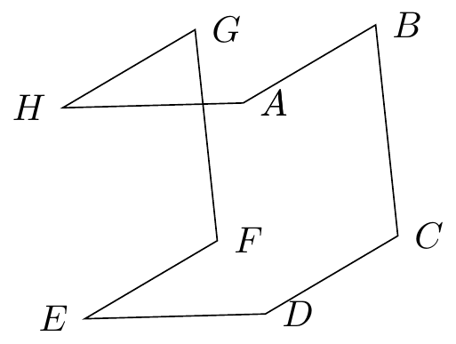
Fig. 16.27: cube rotate around

https://tex.stackexchange.com/questions/388621/optimizing-perspective-tikz-graphic

\usetikzlibrary{patterns}
\usetikzlibrary{3d,calc}
\begin{tikzpicture}[y={(.5cm,.7cm)}]
  \coordinate (A) at ( 1, 1, 1);
  \coordinate (B) at ( 1, 1,-1);
  \coordinate (C) at ( 1,-1,-1);
  \coordinate (D) at ( 1,-1, 1);
  \coordinate (E) at (-1,-1, 1);
  \coordinate (F) at (-1,-1,-1);
  \coordinate (G) at (-1, 1,-1);
  \coordinate (H) at (-1, 1, 1);
  \draw (A) node[right=1pt] {$A$}--
        (B) node[right=1pt] {$B$}--
        (C) node[right=1pt] {$C$}--
        (D) node[right=1pt] {$D$}--
        (E) node[left= 1pt] {$E$}--
        (F) node[right=1pt] {$F$}--
        (G) node[right=1pt] {$G$}--
        (H) node[left= 1pt] {$H$}--
        (A) node[right=1pt] {$A$};
\end{tikzpicture}

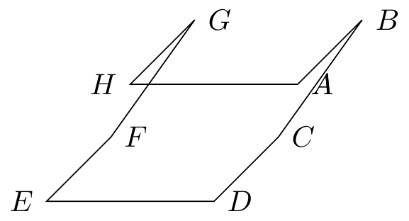
Fig. 16.28: cube perspective slant

https://github.com/XiangyunHuang/bookdown-broken/blob/master/index.Rmd

\smartdiagramset{planet color=gray!40!white, 
uniform color list=gray!40!white for 10 items}
\smartdiagram[bubble diagram]{Basic skills,
  Edit~/\\ (RStudio), 
  Organize~/\\ (bookdown), 
  Cooperate~/\\ (Git), 
  Typeset~/\\ (LaTeX/Pandoc), 
  Compile~/\\ (GitHub Action)}

Fig. 16.29: modern statistics plot skills

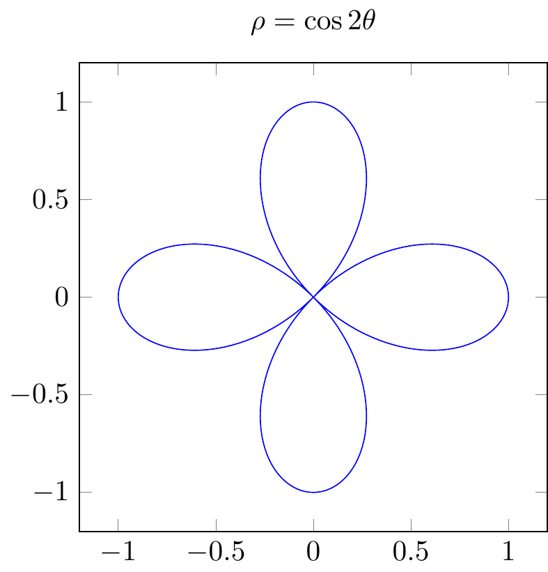
16.3 plots of functions

https://tikz.dev/tikz-plots

A warning before we get started: If you are looking for an easy way to create a normal plot of a function with scientific axes, ignore this section and instead look at the pgfplots package or at the datavisualization command from Part VI.

https://tikz.dev/tikz-plots#sec-22.5

\begin{tikzpicture}[domain=0:4]
  \draw[very thin,color=gray] (-0.1,-1.1) grid (3.9,3.9);

  \draw[->] (-0.2,0) -- (4.2,0) node[right] {$x$};
  \draw[->] (0,-1.2) -- (0,4.2) node[above] {$f(x)$};

  \draw[color=red]    plot (\x,\x)             node[right] {$f(x) =x$};
  % \x r means to convert '\x' from degrees to _r_adians:
  \draw[color=blue]   plot (\x,{sin(\x r)})    node[right] {$f(x) = \sin x$};
  \draw[color=orange] plot (\x,{0.05*exp(\x)}) node[right] {$f(x) = \frac{1}{20} \mathrm e^x$};
\end{tikzpicture}

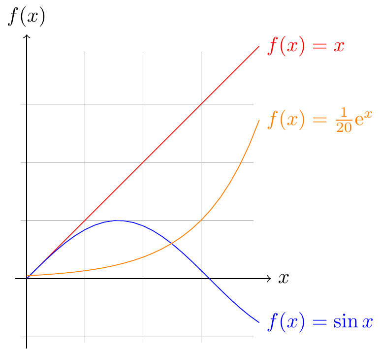
Fig. 16.30: plots of functions

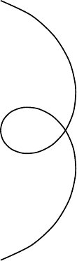
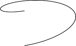
\tikz \draw[scale=0.5,domain=-3.141:3.141,smooth,variable=\t]
  plot ({\t*sin(\t r)},{\t*cos(\t r)});

Fig. 16.31: 2D parametric function

\tikz \draw[domain=0:360,
            smooth,
            variable=\t]
  plot ({sin(\t)},\t/360,{cos(\t)});

Fig. 16.32: 3D parametric function

16.4 commutative diagram

cd = CD = commutative diagram

tikz-cd = TikZ-CD

\usetikzlibrary{cd} vs. usepackage{tikz-cd}

https://tex.stackexchange.com/questions/546392/usepackagetikz-cd-vs-usetikzlibrarycd

No (practical) difference. The code (excluding copyright comment lines) in tikz-cd.sty is
\ProvidesPackage{tikz-cd}[2014/10/30 v0.9e Commutative diagrams with tikz]
\RequirePackage{tikz}[2013/12/13] % pgf version 3.0.0 required
\usetikzlibrary{cd}

\endinput

Never put \begin{tikzcd} inside \begin{tikzpicture}

https://tex.stackexchange.com/questions/425296/half-of-tikzcd-diagram-is-missing

\usetikzlibrary{cd,arrows.meta}
\begin{tikzcd}
11 & 12 & 13 \\
21 & 22 & 23 \\
31 & 32 & 33
\end{tikzcd}

Fig. 16.33: learn TikZ-CD or tikz-cd in one picture

\usetikzlibrary{cd,arrows.meta}
\begin{tikzcd}
11
&
12
&
13
\\
21
&
22
&
23
\\
31
&
32
&
33
\end{tikzcd}

Fig. 16.34: TikZ-CD or tikz-cd matrix nodes

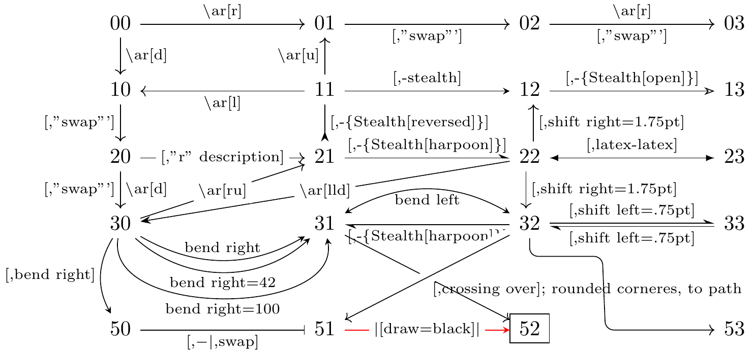
Fig. 16.35: TikZ-CD or tikz-cd matrix nodes expanded longitudinally

\usetikzlibrary{cd,arrows.meta}
\begin{tikzcd}[column sep=2.75cm]%small,large,huge
00
\ar[r,"\backslash \text{ar[r]}"]
\ar[d,"\backslash \text{ar[d]}"]
&
01
\ar[r,"\text{[,"swap"']}"']
&
02
\ar[r,"\backslash \text{ar[r]}","\text{[,"swap"']}"']
&
03
\\
10
\ar[d,"\text{[,"swap"']}"']
&
11
\ar[u,"\backslash \text{ar[u]}"]
\ar[l,"\backslash \text{ar[l]}"]
\ar[r,-stealth,"\text{[,-}\text{stealth}\text{]}"]
\ar[d,-{Stealth[reversed]},"\text{[,-}\{\text{Stealth[reversed]}\}\text{]}"]
&
12
\ar[r,-{Stealth[open]},"\text{[,-}\{\text{Stealth[open]}\}\text{]}"]
&
13
\\
20
\ar[r,"\text{[,"r" description]}" description]
\ar[d,"\backslash \text{ar[d]}","\text{[,"swap"']}"']
&
21
\ar[r,-{Stealth[harpoon]},"\text{[,-}\{\text{Stealth[harpoon]}\}\text{]}"]
&
22
\ar[u,shift right=1.75pt,"\text{[,shift right=1.75pt]}"']
\ar[lld,-Stealth,"\backslash \text{ar[lld]}" description]
\ar[r,latex-latex,"\text{[,latex-latex]}"]
\ar[d,shift right=1.75pt,"\text{[,shift right=1.75pt]}"]
&
23
\\
30
\ar[ru,"\backslash \text{ar[ru]}" description]
\ar[r,bend right,-stealth,"\text{bend right}"]
\ar[r,bend right=42,-stealth,"\text{bend right=42}"']
\ar[r,bend right=100,-stealth,"\text{bend right=100}"']
\ar[dd,bend right,-stealth,"\text{[,bend right]}"']
&
31
\ar[r,bend left,stealth-stealth,"\text{bend left}"']
\ar[ddr]
&
32
\ar[l,-{Stealth[harpoon]},"\text{[,-}\{\text{Stealth[harpoon]}\}\text{]}"]
\ar[r,-{Stealth[harpoon]},shift left=.75pt,"\text{[,shift left=.75pt]}"]
\ar[ddl,crossing over,"\text{[,crossing over]; rounded corneres, to path}"]
\ar[ddr,
    rounded corners,
    to path={--([yshift=-2ex]\tikztostart.south)
              --([yshift=-2ex,xshift=+2ex]\tikztostart.south)
              --([yshift=-2ex,xshift=+8ex]\tikztostart.south)
              --([xshift=-12ex]\tikztotarget.west)
              --(\tikztotarget)
             },
    ]
&
33
\ar[l,-{Stealth[harpoon]},shift left=.75pt,"\text{[,shift left=.75pt]}"]
\\
&
&
&
\\
50
\ar[r,-|,"\text{[,}-|\text{,swap]}",swap]
&
51
\ar[r,-stealth,red,text=black,"|\text{[draw=black]}|" description]
&
|[draw=black]|52
&
53
\end{tikzcd}

Fig. 16.36: learn TikZ-CD or tikz-cd in one picture

https://tex.stackexchange.com/questions/515267/how-can-i-make-arrows-touch-boxed-expressions-in-tikzcd

cells={nodes={draw}}

in

\begin{tikzcd}[column sep=2.75cm, %small,large,huge
                     cells={nodes={draw}}
                    ]

Fig. 16.37: learn TikZ-CD or tikz-cd in one picture 2

\usetikzlibrary{cd,arrows.meta}
\begin{tikzcd}[column sep=2.75cm, %small,large,huge
                     cells={nodes={draw}}
                    ]
00
\ar[r,"\backslash \text{ar[r]}"]
\ar[d,"\backslash \text{ar[d]}"]
&
01
\ar[r,"\text{[,"swap"']}"']
&
02
\ar[r,"\backslash \text{ar[r]}","\text{[,"swap"']}"']
&
03
\\
10
\ar[d,"\text{[,"swap"']}"']
&
11
\ar[u,"\backslash \text{ar[u]}"]
\ar[l,"\backslash \text{ar[l]}"]
\ar[r,-stealth,"\text{[,-}\text{stealth}\text{]}"]
\ar[d,-{Stealth[reversed]},"\text{[,-}\{\text{Stealth[reversed]}\}\text{]}"]
&
12
\ar[r,-{Stealth[open]},"\text{[,-}\{\text{Stealth[open]}\}\text{]}"]
&
13
\\
20
\ar[r,"\text{[,"r" description]}" description]
\ar[d,"\backslash \text{ar[d]}","\text{[,"swap"']}"']
&
21
\ar[r,-{Stealth[harpoon]},"\text{[,-}\{\text{Stealth[harpoon]}\}\text{]}"]
&
22
\ar[u,shift right=1.75pt,"\text{[,shift right=1.75pt]}"']
\ar[lld,-Stealth,"\backslash \text{ar[lld]}" description]
\ar[r,latex-latex,"\text{[,latex-latex]}"]
\ar[d,shift right=1.75pt,"\text{[,shift right=1.75pt]}"]
&
23
\\
30
\ar[ru,"\backslash \text{ar[ru]}" description]
\ar[r,bend right,-stealth,"\text{bend right}"]
\ar[r,bend right=42,-stealth,"\text{bend right=42}"']
\ar[r,bend right=100,-stealth,"\text{bend right=100}"']
\ar[dd,bend right,-stealth,"\text{[,bend right]}"']
&
31
\ar[r,bend left,stealth-stealth,"\text{bend left}"']
\ar[ddr]
&
32
\ar[l,-{Stealth[harpoon]},"\text{[,-}\{\text{Stealth[harpoon]}\}\text{]}"]
\ar[r,-{Stealth[harpoon]},shift left=.75pt,"\text{[,shift left=.75pt]}"]
\ar[ddl,crossing over,"\text{[,crossing over]; rounded corneres, to path}"]
\ar[ddr,
    rounded corners,
    to path={--([yshift=-2ex]\tikztostart.south)
              --([yshift=-2ex,xshift=+2ex]\tikztostart.south)
              --([yshift=-2ex,xshift=+8ex]\tikztostart.south)
              --([xshift=-12ex]\tikztotarget.west)
              --(\tikztotarget)
             },
    ]
&
33
\ar[l,-{Stealth[harpoon]},shift left=.75pt,"\text{[,shift left=.75pt]}"]
\\
&
&
&
\\
50
\ar[r,-|,"\text{[,}-|\text{,swap]}",swap]
&
51
\ar[r,-stealth,red,text=black,"|\text{[draw=none]}|" description]
&
|[draw=none]|52
&
53
\end{tikzcd}

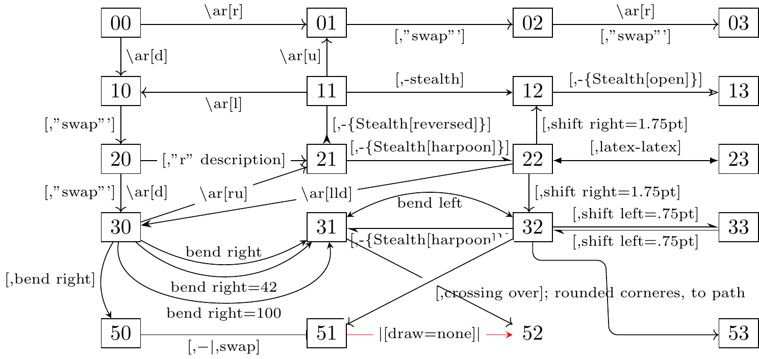
Fig. 16.38: learn TikZ-CD or tikz-cd in one picture 2

https://tex.stackexchange.com/questions/484743/format-single-node-in-tikzcd

\usetikzlibrary{cd,arrows.meta,shapes}
\begin{tikzcd}[cells={nodes={draw=black,ellipse}}]
0 \ar[r] & 1 \ar[r] & |[draw=none]|\dots \ar[r] & n-1 \ar[r] & n
\end{tikzcd}

Fig. 16.39: individual node without drawing margin

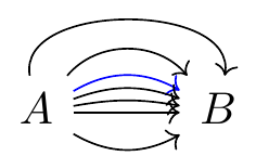
https://tex.stackexchange.com/questions/586160/drawing-commutative-diagram-with-encircled-nodes-in-tikz-cd-package

\usetikzlibrary{cd,fit,shapes.geometric}
\tikzset{E/.style = {ellipse, draw=blue, dashed,
                    inner xsep=-2mm,inner ysep=-4mm,
                    rotate=-30,fit=#1
                   }
        }
\begin{tikzcd}[arrows = dash,
                execute at end picture = {
                \node[E = (tikz@f@1-2-2) (tikz@f@1-3-3)] {};
                \node[E = (tikz@f@1-3-1) (tikz@f@1-4-2)] {};
                        }% end of execute at end picture
              ]
    &   R   \ar[d]  &   \\
    &   A+B \ar[dl] \ar[dr] &   \\
A   \ar[dr] &   &   B   \ar[dl] \\
    &   A \cap B    &
\end{tikzcd}

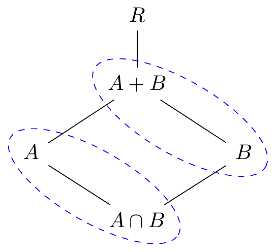
Fig. 16.40: enclosed nodes

box in TikZ-CD^[16.4.3]

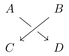
\usetikzlibrary{cd,arrows.meta}
\begin{tikzcd}
A \ar[r,-stealth,"f","g"'] \ar[d,-{Stealth[harpoon]},shift left=0.5pt,"\varphi"] \ar[rr,-stealth,bend left] & B & E \\
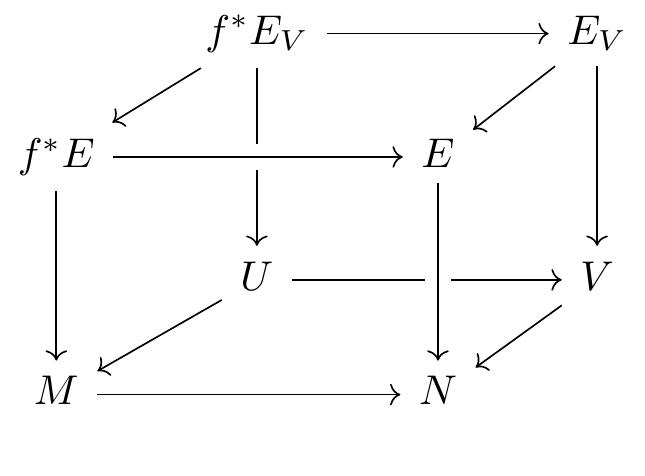
C \ar[r,-latex,"g"'] \ar[u,-{Stealth[harpoon]},shift left=0.5pt,"\varphi^{{\scriptscriptstyle -1}}"] \ar[d,harpoon,shift left=0.5pt,"\varphi"] & D & F \\
G \ar[r,"f"] \ar[u,harpoon,shift left=0.5pt,"\varphi^{-1}"] & H \ar[uur,-stealth,"\phi" description]
\end{tikzcd}

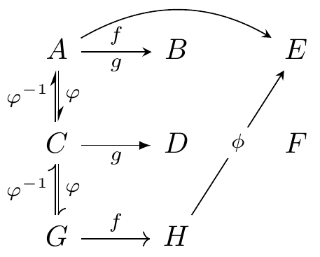
Fig. 16.41: TikZ-CD or tikz-cd + arrows.meta

\usetikzlibrary{cd,arrows.meta}
\begin{tikzcd}
A \ar[r,-{Stealth[harpoon,swap,open]}] & B
\end{tikzcd}

Fig. 16.42: TikZ-CD or tikz-cd + arrows.meta

TikZcd editor

https://github.com/yishn/tikzcd-editor

https://tikzcd.yichuanshen.de/

https://darknmt.github.io/res/tikzcd-editor/

tikz-cd @ CTAN(Comprehensive TEX Archive Network)

https://ctan.org/tex-archive/graphics/pgf/contrib/tikz-cd

tikzcd manual

https://ctan.mirror.twds.com.tw/tex-archive/graphics/pgf/contrib/tikz-cd/tikz-cd-doc.pdf

16.4.1 arrows

https://latexdraw.com/exploring-tikz-arrows/

16.4.1.1 predefined arrow tip in TikZ

16.4.1.1.1 stealth arrow tip

-stealth without capital S = -{Stealth} in arrows.meta

\begin{tikzpicture}
  \node at (0, 0) {};
    \draw [-stealth]        (0, 0) -- (1, 0);
    \draw [stealth-]        (0,-1) -- (1,-1);
    \draw [stealth-stealth] (0,-2) -- (1,-2);
  \node at (0,-2) {};
\end{tikzpicture}

Fig. 16.43: stealth arrow tip

16.4.1.1.2 reversed stealth arrow tip

-stealth reversed = -{Stealth[reversed]} in arrows.meta

\begin{tikzpicture}
  \node at (0, 0) {};
    \draw [-stealth reversed]                 (0, 0) -- (1, 0);
    \draw [stealth reversed-]                 (0,-1) -- (1,-1);
    \draw [stealth reversed-stealth reversed] (0,-2) -- (1,-2);
  \node at (0,-2) {};
\end{tikzpicture}

Fig. 16.44: reversed stealth arrow tip

16.4.1.1.3 to arrow tip

-to

\begin{tikzpicture}
  \node at (0, 0) {};
    \draw [-to]   (0, 0) -- (1, 0);
    \draw [to-]   (0,-1) -- (1,-1);
    \draw [to-to] (0,-2) -- (1,-2);
  \node at (0,-2) {};
\end{tikzpicture}

Fig. 16.45: to arrow tip

16.4.1.1.4 latex arrow tip

-latex with flat-tailed arrow head, differing from -stealth

\begin{tikzpicture}
  \node at (0, 0) {};
    \draw [-latex]      (0, 0) -- (1, 0);
    \draw [latex-]      (0,-1) -- (1,-1);
    \draw [latex-latex] (0,-2) -- (1,-2);
  \node at (0,-2) {};
\end{tikzpicture}

Fig. 16.46: to arrow tip

16.4.1.1.5 | arrow tip

-| like inhibition in biological pathway

\begin{tikzpicture}
  \node at (0, 0) {};
    \draw [-|]  (0, 0) -- (1, 0);
    \draw [|-]  (0,-1) -- (1,-1);
    \draw [|-|] (0,-2) -- (1,-2);
  \node at (0,-2) {};
\end{tikzpicture}

Fig. 16.47: to arrow tip

16.4.1.2 arrows.meta

customizing arrow heads

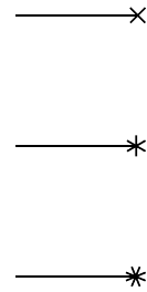
16.4.1.2.1 reversing, halving, swapping, opening

https://tikz.dev/tikz-arrows#sec-16.3.5

\usetikzlibrary{arrows.meta}
\begin{tikzpicture}
  \node at (0, 0) {};
    \draw [-{Stealth[reversed]}]      (0, 0) -- (1, 0);
    \draw [-{Stealth[harpoon]}]       (0,-1) -- (1,-1);
    \draw [-{Stealth[harpoon,swap]}]  (0,-2) -- (1,-2);
  \draw [-{Stealth[open]}]          (0,-3) -- (1,-3);
  \node at (0,-2) {};
\end{tikzpicture}

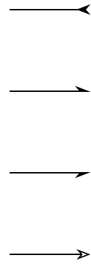
Fig. 16.48: reversing, halving, swapping, opening

16.4.1.2.2 mathematical arrows

Classical TikZ Rightarrow
Computer Modern Rightarrow
Implies
To

\usetikzlibrary{arrows.meta}
\begin{tikzpicture}
  \node at (0, 0) {};
    \draw [-{Classical TikZ Rightarrow}]  (0, 0) -- (1, 0);
    \draw [-{Computer Modern Rightarrow}] (0,-1) -- (1,-1);
    \draw [-{Implies},double]             (0,-2) -- (1,-2);
  \draw [-To]                           (0,-3) -- (1,-3);
  \node at (0,-3) {};
\end{tikzpicture}

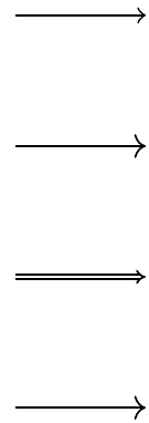
Fig. 16.49: mathematical arrows

16.4.1.2.3 ray arrow tip

-Rays

\usetikzlibrary{arrows.meta}
\begin{tikzpicture}
  \node at (0, 0) {};
    \draw [-Rays]         (0, 0) -- (1, 0);
    \draw [-{Rays[n=6]}]  (0,-1) -- (1,-1);
    \draw [-{Rays[n=8]}]  (0,-2) -- (1,-2);
  \node at (0,-2) {};
\end{tikzpicture}

Fig. 16.50: Ray arrow tip

16.4.1.2.4 arrow head scale

e.g. -{Stealth[scale=2]}

\usetikzlibrary{arrows.meta}
\begin{tikzpicture}
  \node at (0, 0) {};
    \draw [-stealth]            (0, 0) -- (1, 0);
    \draw [-{Stealth[scale=2]}] (0,-1) -- (1,-1);
  \node at (0,-1) {};
\end{tikzpicture}

Fig. 16.51: arrow head scale

16.4.1.2.5 arrow head size

https://tikz.dev/tikz-arrows#sec-16.3.1

\usetikzlibrary{arrows.meta}
\begin{tikzpicture}
  \node at (0, 0) {};
    \draw [-stealth]                          (0, 0) -- (1, 0);
    \draw [-{Stealth[length=3mm, width=2mm]}] (0,-1) -- (1,-1);
  \node at (0,-1) {};
\end{tikzpicture}

Fig. 16.52: arrow head size

16.4.1.2.6 arrow head slant

e.g. -{Stealth[slant=2]}

\usetikzlibrary{arrows.meta}
\begin{tikzpicture}
  \node at (0, 0) {};
    \draw [-Stealth]               (0, 0) -- (1, 0);
  \draw [-{Stealth[slant=-0.5]}] (0,-1) -- (1,-1);
  \draw [-{Stealth[slant=   1]}] (0,-2) -- (1,-2);
  \node at (0,-2) {};
\end{tikzpicture}

Fig. 16.53: arrow head slant

16.4.1.2.7 arrow head color

e.g.

-{Stealth[color=cyan]}
-{Stealth[fill=red]}
red,-{Stealth}

\usetikzlibrary{arrows.meta}
\begin{tikzpicture}
  \node at (0, 0) {};
    \draw [-stealth]               (0, 0) -- (1, 0);
    \draw [-{Stealth[color=cyan]}] (0,-1) -- (1,-1);
  \draw [-{Stealth[fill=red]}  ] (0,-2) -- (1,-2);
  \draw [red,-{Stealth}        ] (0,-3) -- (1,-3);
  \node at (0,-3) {};
\end{tikzpicture}

Fig. 16.54: arrow and arrow head color

16.4.1.2.8 multiple arrow head

e.g. -{Stealth}{Stealth}{Stealth}

\usetikzlibrary{arrows.meta}
\begin{tikzpicture}
  \node at (0, 0) {};
    \draw [-stealth]                     (0, 0) -- (1, 0);
    \draw [-{Stealth}{Stealth}{Stealth}] (0,-1) -- (1,-1);
  \node at (0,-1) {};
\end{tikzpicture}

Fig. 16.55: multiple arrow head

16.4.1.3 default stealth arrow

https://tex.stackexchange.com/questions/113437/stealth-arrow-in-math

\usetikzlibrary{cd,arrows}
\tikzset{
  commutative diagrams/.cd, 
  arrow style=tikz, 
  diagrams={>=stealth}
}
\begin{tikzcd}
A \ar[r,"f"] \ar[d,harpoon,shift left=0.5pt,"\varphi"] \ar[rr,bend left] & B & E \\
C \ar[r] \ar[u,harpoon,shift left=0.5pt,"\varphi^{-1}"] & D & F \\
G & H \ar[uur,-stealth]
\end{tikzcd}

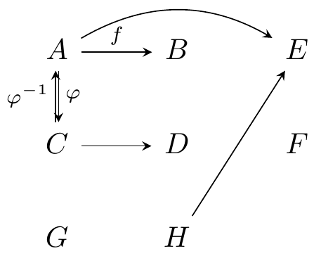
Fig. 16.56: default stealth arrow

16.4.1.4 harpoon

harpoon ~ half arrow

https://tex.stackexchange.com/questions/715462/rightleftharpoons-in-commutative-diagram

\usetikzlibrary{cd}
\begin{tikzcd}
cc \ar[r,shift left=1pt,harpoon,"a"] \ar[d,shift left=1pt,harpoon,"r"] &
ct \ar[l,shift left=1pt,harpoon,"b"] \ar[d,shift left=1pt,harpoon,"r"]
\\
tc \ar[r,shift left=1pt,harpoon,"a"] \ar[u,shift left=1pt,harpoon,"l"] &
tt \ar[l,shift left=1pt,harpoon,"b"] \ar[u,shift left=1pt,harpoon,"l"]
\end{tikzcd}

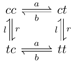
Fig. 16.57: harpoon in cd

16.4.1.5 bend

https://tex.stackexchange.com/questions/354480/very-curved-arrow-with-tikzcd

\usetikzlibrary{cd}
\begin{tikzcd}
A
\ar[r]
\ar[r, bend right]
\ar[r, bend left, blue]
\ar[r, bend left=10]
\ar[r, bend left=20]
\ar[r, bend left=50]
\ar[r, bend left=100]
& B
\end{tikzcd}

Fig. 16.58: arrow bend

16.4.1.6 rounded corners

https://tex.stackexchange.com/questions/295428/rounded-arrow-in-tikzcd-with-text-on-it

\usetikzlibrary{cd,positioning}
\begin{tikzcd}[sep=large, execute at end picture={\node[below = 1mm of tikz@f@1-1-2] {$\scriptstyle  g' \circ g$};}]
    B \ar{r}[swap]{g\vphantom{'}}
    \ar[to path={--([yshift=-4ex]\tikztostart.south)
                 -|(\tikztotarget)},rounded corners=12pt]{rr}
    & B' \ar{r}[swap]{g'} & B''
\end{tikzcd}

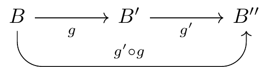
Fig. 16.59: rounded corners

16.4.1.7 crossing over

\usetikzlibrary{cd}
\begin{tikzcd}
 A \ar[dr] & B \ar[dl, crossing over] \\
 C
 & D
 \end{tikzcd}

Fig. 16.60: crossing over

\usetikzlibrary{cd}
\begin{tikzcd}[row sep=scriptsize, column sep=scriptsize]
 & f^* E_V \ar[dl] \ar[rr] \ar[dd] & & E_V \ar[dl] \ar[dd] \\
 f^* E \ar[rr, crossing over] \ar[dd] & & E \\
 & U \ar[dl] \ar[rr] & & V \ar[dl] \\
 M \ar[rr] & & N \ar[from=uu, crossing over]\\
 \end{tikzcd}

Fig. 16.61: pseudo 3D diagram

16.4.1.8 tweaking to paths

\usetikzlibrary{cd}
\begin{tikzcd}
  A \ar[dr, controls={+(1.5,0.5) and +(-1,0.8)}]
    \ar[dr, dashed, to path=|- (\tikztotarget)]
    & \\
    & B \ar[loop right]
\end{tikzcd}

Fig. 16.62: crossing over

\usetikzlibrary{cd}
\begin{tikzcd}
  A \ar[r]
    & B \ar[r]
        \ar[d, phantom,""{coordinate,name=Z}]
    & C \ar[dll,
               "\delta",
               rounded corners,
               to path={--([xshift=2ex]\tikztostart.east)
                        |-(Z)[near end]\tikztonodes
                        -|([xshift=-2ex]\tikztotarget.west)
                        --(\tikztotarget)}] \\
  D \ar[r]
    & E \ar[r]
    & F
\end{tikzcd}

Fig. 16.63: crossing over

\usetikzlibrary{cd}
\begin{tikzcd}
  A \ar[r]
    & B \ar[r]
    & C \ar[dll,
               "\delta",
               rounded corners,
               to path={--([xshift=2ex]\tikztostart.east)
                        --([xshift=-2ex]\tikztotarget.west)
                        --(\tikztotarget)}] \\
  D \ar[r]
    & E \ar[r]
    & F
\end{tikzcd}

Fig. 16.64: crossing over

16.4.2 label

https://tex.stackexchange.com/questions/477733/two-labels-up-and-down-for-same-arrow

\usetikzlibrary{cd}
\begin{tikzcd}%              V
A \ar[r, "\alpha", "\beta"'] & B
\end{tikzcd}

Fig. 16.65: labels over and under the arrow

16.4.2.1 single quotation mark to swap

\usetikzlibrary{cd}
\begin{tikzcd}
A \ar[r, "\alpha"] & B
\end{tikzcd}

Fig. 16.66: label over the arrow without single quotation

\usetikzlibrary{cd}
\begin{tikzcd}
A \ar[r, "\alpha"'] & B
\end{tikzcd}

Fig. 16.67: label under the arrow with single quotation

16.4.2.2 swap

\usetikzlibrary{cd}
\begin{tikzcd}
A \ar[r, "\alpha"] & B
\end{tikzcd}

Fig. 16.68: label over the arrow or no swap

\usetikzlibrary{cd}
\begin{tikzcd}
A \ar[r, "\alpha", swap] & B
\end{tikzcd}

Fig. 16.69: label swap under the arrow

16.4.2.3 every arrow swap

https://tex.stackexchange.com/questions/515697/how-can-we-change-the-positions-of-the-labels-on-a-tikz-cd-commutative-diagram

every arrow/.append style={swap}

16.4.3 box in TikZ-CD

https://stackoverflow.com/questions/50392582/box-in-commutative-diagram

https://tex.stackexchange.com/questions/360083/filling-of-diagrams-using-tikzcd/360152#360152

16.4.4 examples

https://tex.stackexchange.com/questions/218274/how-can-i-draw-commutative-diagrams-in-latex

\usetikzlibrary{cd}
\begin{tikzcd}
A \ar{r}{\varphi} \ar[swap]{d}{\varrho_f} & B \ar{d}{\varrho_g} \\%
A_f \ar{r}{\varphi_f}& B_g
\end{tikzcd}

Fig. 16.70: commutative diagram example 0

https://tex.stackexchange.com/questions/402572/how-to-make-a-commutative-diagram-using-tikz-cd

\usetikzlibrary{cd}
\begin{tikzcd}[row sep=huge]
A \ar[r,"\phi_n"] \ar[d,swap,"\pi"] &
A_n \ar[r,"\epsilon_{i,n}"] \ar[dl,swap,"\psi_n"] \ar[dr,"\pi_n"] &
M_{n_k}(\mathbb{C}) \ar[d,"\eta_{i,n}"]
\\
B(H) & & B(H_n) \ar[ll,dashed]
\end{tikzcd}

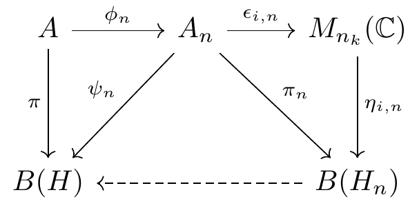
Fig. 16.71: commutative diagram example 1

https://tex.stackexchange.com/questions/115783/how-to-draw-commutative-diagrams

\usetikzlibrary{cd,arrows}
\begin{tikzcd}
A \ar{r}{f} \ar[swap]{dr}{g\circ f} & B \ar{d}{g} \\
& C
\end{tikzcd}

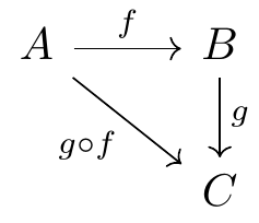
Fig. 16.72: commutative diagram example 2

https://tex.stackexchange.com/questions/414292/tikz-commutative-diagrams-compiling-and-best-practice

\usetikzlibrary{cd}
\begin{tikzcd}
C \ar[d, "\langle f_i \rangle_{i \in I}"', dotted] \ar[rd, "f_i"] &  \\
\prod_{i \in I} A_i \ar[r, "\pi_i"'] & A_i
\end{tikzcd}

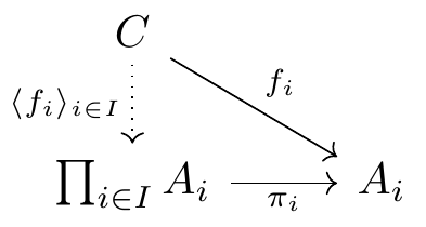
Fig. 16.73: commutative diagram example 3

https://tex.stackexchange.com/questions/483801/mapping-arrows-in-commutative-diagrams

\usetikzlibrary{cd}
\begin{tikzcd}
a \ar[r, maps to] & \phi(a) &[-2em] \\[-4ex]
R\ar[r, hook, "\phi"] \ar[dr, hook, "\iota"] & K & \phi(a) \\
& Q(R) \ar[u, dotted, "\exists ! \Phi"'] & \frac{a}{1} \ar[u, maps to] \\[-10ex]
a \ar[dr, maps to] \\
& \frac{a}{1} & 
\end{tikzcd}

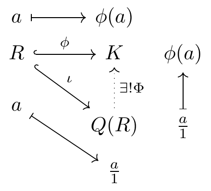
Fig. 16.74: commutative diagram example 4

if not using tikz-cd,

\usetikzlibrary{arrows,positioning}
\begin{tikzpicture}
\node (r) at (0,0) {$R$};
\node (k) at (3,0) {$K$};
\node (q) at (3,-3) {$Q(R)$};
\node (ra) at (0,.8) {$a$};
\node (ka) at (3,.8) {$\phi(a)$};
\node (kb) at (4,0) {$\phi(k)$};
\node (qb) at (4,-3) {$\frac a1$};
\path (q) node[below left=1em and 1em] (qc) {$\frac a1$};
\path (r) node[below left=1em and 1em] (rc) {$a$};
\draw[right hook->] (r)--(k) node[midway,above] {$\scriptstyle\phi$};
\draw[right hook->] (r)--(q) node[midway,above right] {$\scriptstyle\iota$};
\draw[dotted,->] (q)--(k) node[midway,right] {$\scriptstyle\exists!\Phi$};
\draw[|->] (ra) edge (ka) (qb) edge (kb) (rc) edge (qc);
\end{tikzpicture}

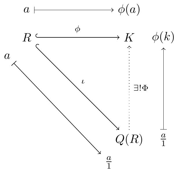
Fig. 16.75: commutative diagram example 4 not using tikz-cd

separated diagrams with tikz-cd,

\usetikzlibrary{cd}
\begin{tikzcd}
R\ar[r, hook, "\phi"] \ar[dr, hook, "\iota"] & K &
a \ar[r, maps to,"\phi"] \ar[dr, maps to,"\iota"] & \phi(a) \\
& Q(R) \ar[u, dotted, "\exists ! \Phi"'] &
& \frac{a}{1} \ar[u, maps to,"\Phi"']
\end{tikzcd}

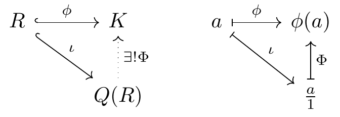
Fig. 16.76: commutative diagram example 4

https://tex.stackexchange.com/questions/510088/tikz-register-map

16.4.5 put a commutative diagram in a nodepart in a tikzpicture

https://tex.stackexchange.com/questions/524955/put-a-commutative-diagram-in-a-nodepart-in-a-tikzpicture/525046#525046

16.5 PGFplots

axis similar to matplotlib figure anatomy, see Fig: 30.1

https://tikz.dev/pgfplots/

https://tikz.dev/pgfplots/tutorial1

Not so common is \pgfplotsset{compat=1.5} . A statement like this should always be used in order to (a) benefit from a more or less recent feature set and (b) avoid changes to your picture if you recompile it with a later version of pgfplots.

\pgfplotsset{width=7cm,compat=1.18}
\begin{tikzpicture}
\begin{axis}[
]
    % density of Normal distribution:
    \addplot [
        red,
        domain=-3e-3:3e-3,
        samples=201,
    ]
        {exp(-x^2 / (2e-3^2)) / (1e-3 * sqrt(2*pi))};
\end{axis}
\end{tikzpicture}

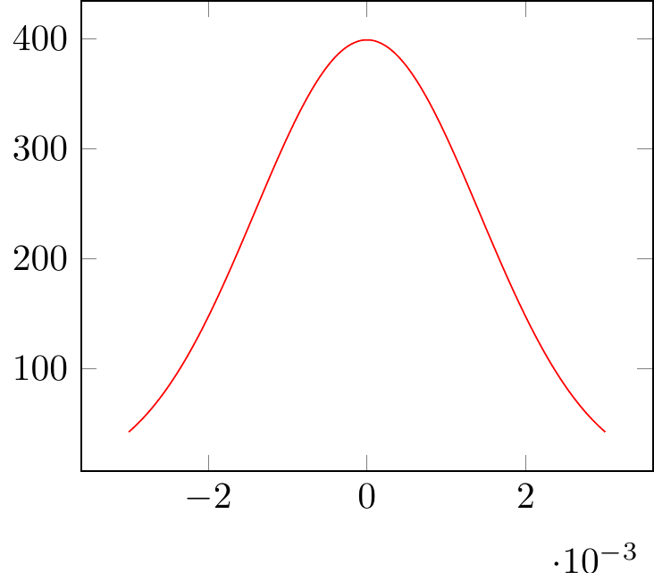
Fig. 16.77: PGFplots: normal distribution

16.5.1 the axis environments

https://tikz.dev/pgfplots/reference-axis

\pgfplotsset{every linear axis/.append style={...}}

\begin{tikzpicture}
    \begin{axis}[
        no markers,
        axis x line = center,
        axis y line = center,
        xlabel = {$ x $}, xlabel style = {right},
        ylabel = {$ y $}, ylabel style = {above},
        xmin = -8, xmax = 8,
        ymin = 0, ymax = 0.45,
        hide obscured x ticks=false, % for origin x tick label i.e. xtick = {0}
        xtick={-4, 0,  4},
        xticklabels={$ \mu_{\scriptscriptstyle{1}} $, 
                    $ \mu_{\scriptscriptstyle{0}} $, 
                    $ \mu_{\scriptscriptstyle{1}} $},
        %extra x ticks={0},
        ytick = \empty,
        x = 1cm, y = 5cm, % x y scaling
        %grid = major,
        domain = -10:10,
        samples = 1000      
    ]
  \end{axis}
\end{tikzpicture}

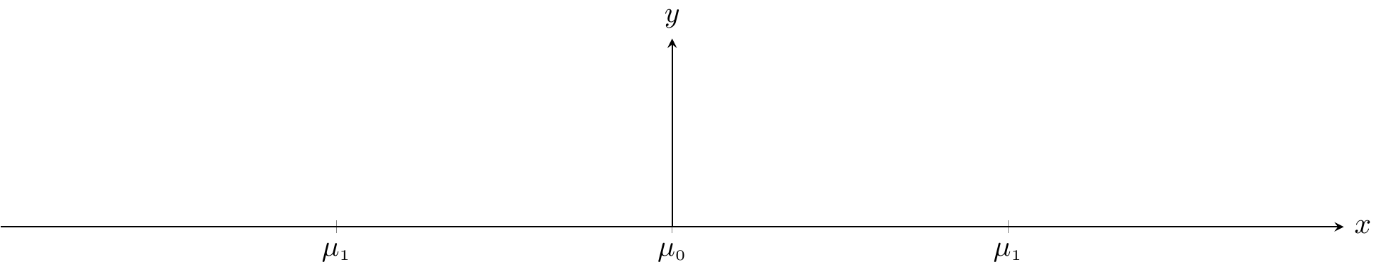
Fig. 16.78: begin{axis}

https://tex.stackexchange.com/questions/134959/axis-lines-middle-and-axis-lines-center

No, there is no difference.

16.5.2 axis descriptions

https://tikz.dev/pgfplots/reference-axisdescription

16.5.2.1 placement of axis descriptions

16.5.2.1.1 coordinate system `axis description cs`

https://tikz.dev/pgfplots/reference-axisdescription#pgfp.axis_description_cs

\addplot {x}; can change to \addplot {x^2}; still with auto blue dots

small dot style,pin=angle:LaTeX label at PGFplots axis coordinate system ;

\begin{tikzpicture}
    \tikzset{
        every pin/.style={fill=yellow!50!white,rectangle,rounded corners=3pt,font=\tiny},
        small dot/.style={fill=black,circle,scale=0.3},
    }
    \begin{axis}[
        clip=false,
        title=How \texttt{axis description cs} works,
    ]
        \addplot {x};
        %small dot style,pin=angle:LaTeX label   at PGFplots axis coordinate system  ;
        \node [small dot,pin=120:{$(0,0)$}]      at (axis description cs:0,0)      {};
        \node [small dot,pin=-30:{$(1,1)$}]      at (axis description cs:1,1)      {};
        \node [small dot,pin=-90:{$(1.03,0.5)$}] at (axis description cs:1.03,0.5) {};
        \node [small dot,pin=125:{$(0.5,0.5)$}]  at (axis description cs:0.5,0.5)  {};
    \end{axis}
\end{tikzpicture}

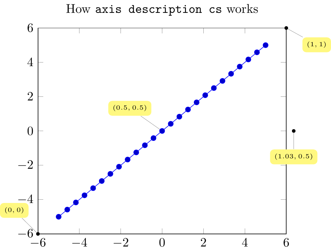
Fig. 16.79: PGFplots: $x$

\begin{tikzpicture}
    \tikzset{
        every pin/.style={fill=yellow!50!white,rectangle,rounded corners=3pt,font=\tiny},
        small dot/.style={fill=black,circle,scale=0.3},
    }
    \begin{axis}[
        clip=false,
        title=How \texttt{axis description cs} works,
    ]
        \addplot {x^2};
        %small dot style,pin=angle:LaTeX label   at PGFplots axis coordinate system  ;
        \node [small dot,pin=120:{$(0,0)$}]      at (axis description cs:0,0)      {};
        \node [small dot,pin=-30:{$(1,1)$}]      at (axis description cs:1,1)      {};
        \node [small dot,pin=-90:{$(1.03,0.5)$}] at (axis description cs:1.03,0.5) {};
        \node [small dot,pin=125:{$(0.5,0.5)$}]  at (axis description cs:0.5,0.5)  {};
    \end{axis}
\end{tikzpicture}

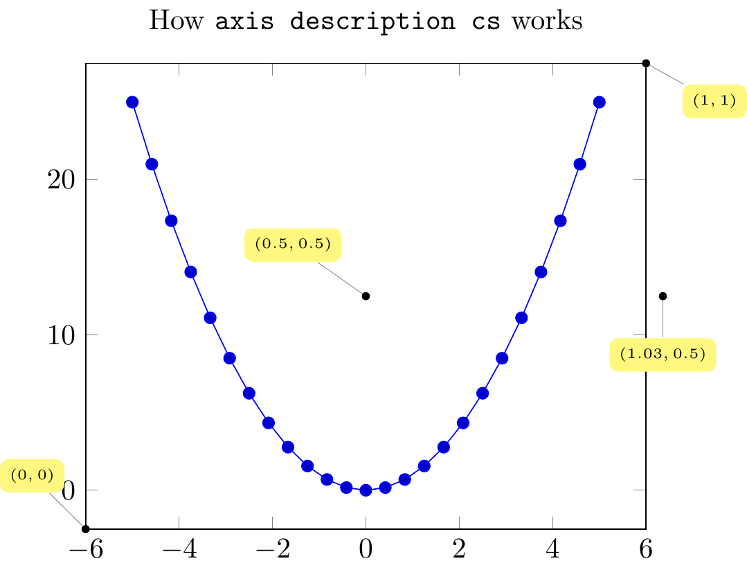
Fig. 16.80: PGFplots: $x^2$

\begin{tikzpicture}
\begin{axis}[
    declare function={
        C=4;
        square(\t)=(\t)^2 + C;
        },
    ]
    \addplot+ [samples=2] {C*x};
    \addplot {square(x)};
\end{axis}
\end{tikzpicture}

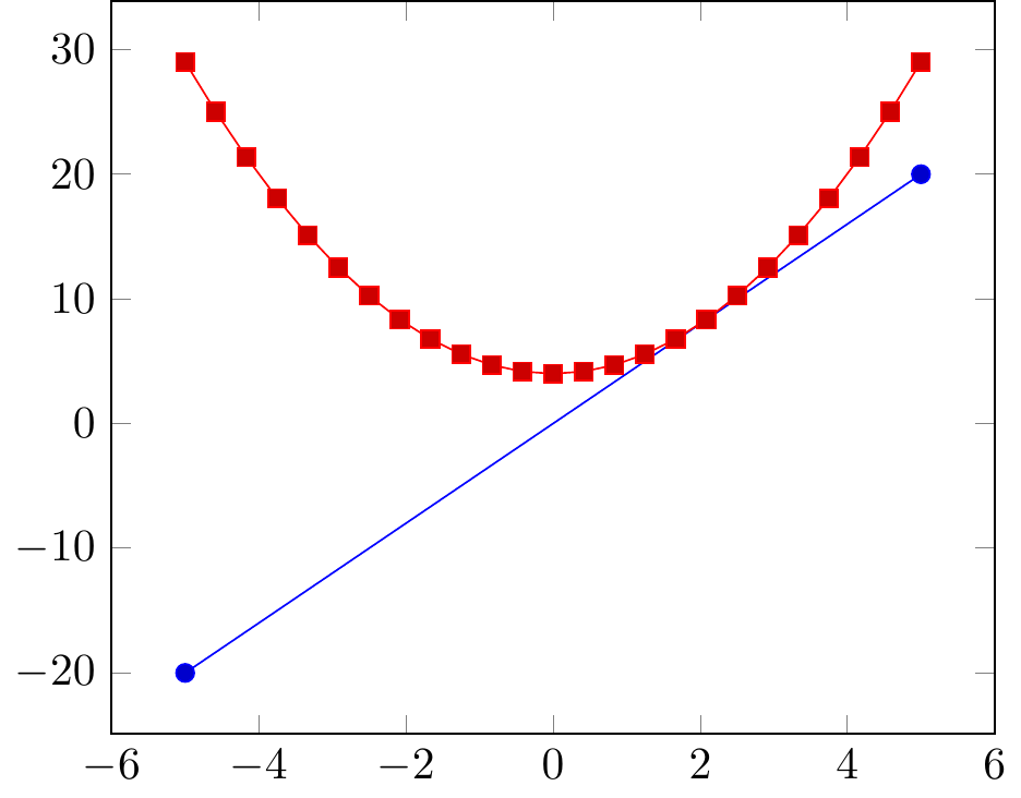
Fig. 16.81: declare function

16.5.3.1 `pgfmathparse`

https://tikz.dev/math-parsing

https://tikz.dev/math-parsing#sec-94.1

This macro parses and returns the result without units in the macro . Example: \pgfmathparse{2pt+3.5pt} will set \pgfmathresult to the text 5.5.

\pgfmathsqrt{x} = \pgfmathparse{sqrt(x)}

\pgfmathln{x} = \pgfmathparse{ln(x)}

…

16.5.3.2 `pgfmathdeclarefunction`

like pgfplotsinvokeforeach

replaces any occurrence of #1 inside of (math image)command(math image) once for every element in (math image)list(math image). Thus, it actually assumes that (math image)command(math image) is like a \newcommand body.

% pgfmathdeclarefunction{name}{num_var}{%
%% #1 = \mu, #2 = \sigma
\pgfmathdeclarefunction{gauss}{2}{%
    \pgfmathparse{1/(#2*sqrt(2*pi))*exp(-((x-#1)^2)/(2*#2^2))}%
}

% pgfmathdeclarefunction{name}{num_var}{%
%% #1 = \mu, #2 = \sigma
\pgfmathdeclarefunction{gauss}{2}{%
    \pgfmathparse{1/(#2*sqrt(2*pi))*exp(-((x-#1)^2)/(2*#2^2))}%
}

\begin{tikzpicture}
    \begin{axis}[
        no markers,
        axis x line = center,
        axis y line = center,
        xlabel = {$ x $}, xlabel style = {right},
        ylabel = {$ y $}, ylabel style = {above},
        xmin = -8, xmax = 8,
        ymin = 0, ymax = 0.45,
        hide obscured x ticks=false, % for origin x tick label i.e. xtick = {0}
        xtick={-4, 0,  4},
        xticklabels={$ \mu_{\scriptscriptstyle{1}} $, 
                    $ \mu_{\scriptscriptstyle{0}} $, 
                    $ \mu_{\scriptscriptstyle{1}} $},
        %extra x ticks={0},
        ytick = \empty,
        x = 1cm, y = 5cm, % x y scaling
        %grid = major,
        domain = -10:10,
        samples = 1000      
    ]
        \addplot [fill=cyan!20, draw=none, domain=-10:-2] {gauss(-4, 1)} \closedcycle;
        \addplot [fill=cyan!20, draw=none, domain=   2:10] {gauss( 4, 1)} \closedcycle;
        \addplot [very thick, cyan!50!black] {gauss(-4, 1)};
        \addplot [very thick, cyan!50!black] {gauss( 0, 1)};
        \addplot [very thick, cyan!50!black] {gauss( 4, 1)};
        %\node [anchor=north] at (axis cs: 0, -0.01) {$ \mu $};
        %\node at (axis cs: -4, -0.02) {$ \mu $};
        \draw [dashed, thin] (axis cs: -4, 0) -- (axis cs: -4, 1);
        \draw [dashed, thin] (axis cs:  4, 0) -- (axis cs: 4, 1);
    \end{axis}
\end{tikzpicture}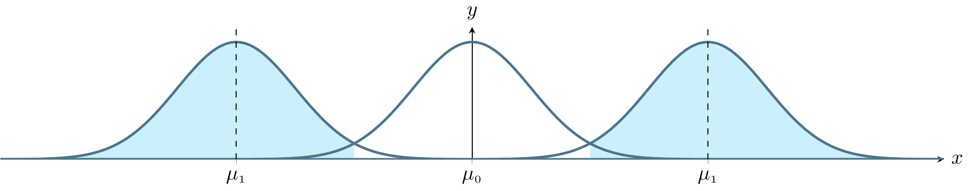

Fig. 16.82: PGFmathDeclareFunction: normal distributions hypothesis testing

https://tex.stackexchange.com/questions/43610/plotting-bell-shaped-curve-in-tikz-pgf

% pgfmathdeclarefunction{name}{num_var}{%
%% #1 = \mu, #2 = \sigma
\pgfmathdeclarefunction{gauss}{2}{%
  \pgfmathparse{1/(#2*sqrt(2*pi))*exp(-((x-#1)^2)/(2*#2^2))}%
}

\begin{tikzpicture}
\begin{axis}[
  no markers, domain=0:10, samples=100,
  axis lines*=left, xlabel=$x$, ylabel=$y$,
  every axis y label/.style={at=(current axis.above origin),anchor=south},
  every axis x label/.style={at=(current axis.right of origin),anchor=west},
  height=5cm, width=12cm,
  xtick={4,6.5}, ytick=\empty,
  enlargelimits=false, clip=false, axis on top,
  grid = major
  ]
  \addplot [fill=cyan!20, draw=none, domain=0:5.96] {gauss(6.5,1)} \closedcycle;
  \addplot [very thick,cyan!50!black] {gauss(4,1)};
  \addplot [very thick,cyan!50!black] {gauss(6.5,1)};
  \draw [yshift=-0.6cm, latex-latex](axis cs:4,0) -- node [fill=white] {$1.96\sigma$} (axis cs:5.96,0);
\end{axis}

\end{tikzpicture}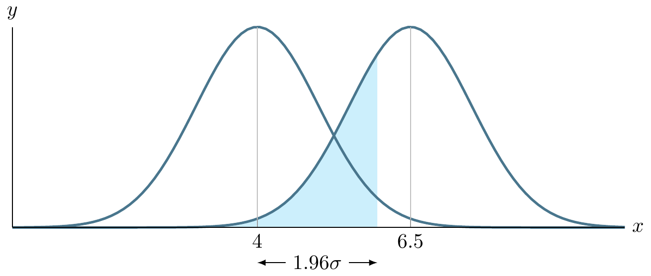

Fig. 16.83: PGFmathDeclareFunction: normal distributions

16.5.4 `|-` and `-|` in TikZ

https://tex.stackexchange.com/questions/401425/tikz-what-exactly-does-the-the-notation-for-arrows-do

(a -| b) where a and b are named nodes or coordinates. This means the coordinate that is at the y-coordinate of a, and x-coordinate of b. Similarly, (a |- b) has the x-coordinate of a and y-coordinate of b.

16.5.5 `pgfplotsinvokeforeach`

https://tikz.dev/pgfplots/pgfplotstable-miscellaneous#\pgfplotsinvokeforeach

like \foreach in TikZ

A variant of \pgfplotsforeachungrouped (and such also of \foreach) which replaces any occurrence of #1 inside of (math image)command(math image) once for every element in (math image)list(math image). Thus, it actually assumes that (math image)command(math image) is like a \newcommand body.

16.5.6 interpolation dashed lines

https://tex.stackexchange.com/questions/193259/what-is-the-easiest-way-to-accomplish-textual-tick-labels-in-tikz

interpa = (10,10), interpb = (30,30), interp = interpolation

({axis cs:0,0}|-interp#1) = (x of (0,0), y of (interpa)) = (0, 10), ...

\begin{tikzpicture}
\begin{axis}[
    axis lines=left,
    xmin = 0, xmax = 40,
    ymin = 0, ymax = 40,
    xtick={10,30},
    xticklabels={$V_i=10$,$V_f=30$},
    ytick={10,30},
    yticklabels={$P_i=10$,$P_f=30$},
    xlabel={Volume},
    ylabel={Pressure}
  ]
  \addplot[very thick,-latex ] coordinates{(10,10) (30,30)}
    % interpa = (10,10), interpb = (30,30), interp = interpolation
    coordinate[at start](interpa)coordinate[at end](interpb);
  \pgfplotsinvokeforeach {a,b} {
    \draw[ultra thin, dashed]
      % ({axis cs:0,0}|-interp#1) = (x of (0,0), y of (interpa)) = (0, 10), ...
      ({axis cs:0,0}|-interp#1)--(interp#1)--(interp#1|-{axis cs:0,0});
    }
\end{axis}
\end{tikzpicture}

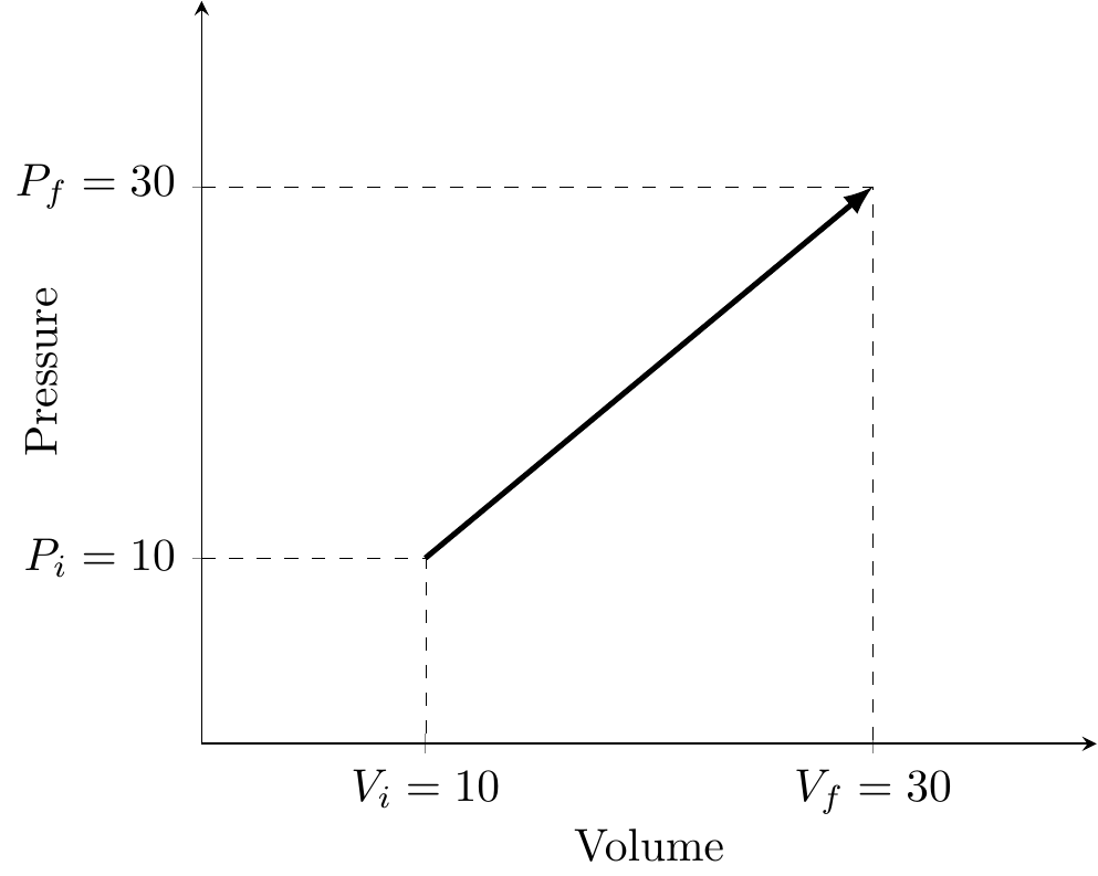
Fig. 16.84: tick texts and interpolation dashed lines

16.5.7 Zewbie

https://zhuanlan.zhihu.com/p/551874337

axis similar to matplotlib figure anatomy, see Fig: 30.1

16.5.7.1 coordinate axis/axes fine-tuing

\begin{tikzpicture}
    \begin{axis}
        % empty
    \end{axis}
\end{tikzpicture}

Fig. 16.85: PGFplots: 2D axis/axes

16.5.7.1.1 range

\begin{tikzpicture}
    \begin{axis}[
        xmin = -1, xmax = 11,
        ymin = -3, ymax = 1,
    ]
        % empty
    \end{axis}
\end{tikzpicture}

Fig. 16.86: PGFplots: axis/axes range

16.5.7.1.2 scaling

axis equal image equivalent to unit vector ratio = {1 1 1}

\begin{tikzpicture}
    \begin{axis}[
        xmin = -1, xmax = 11,
        ymin = -3, ymax = 1,
        axis equal image, % unit vector ratio = {1 1 1},
    ]
        % empty
    \end{axis}
\end{tikzpicture}

Fig. 16.87: PGFplots: axis/axes range

scale only axis

width x axis length, height y axis length

\begin{tikzpicture}
    \begin{axis}[
        xmin = -1, xmax = 11,
        ymin = -3, ymax = 1,
        scale only axis,
        width = 5cm, height = 7cm,
    ]
        % empty
    \end{axis}
\end{tikzpicture}

Fig. 16.88: PGFplots: axis/axes range

x x unit vector length, y y unit vector length

\begin{tikzpicture}
    \begin{axis}[
        xmin = -1, xmax = 11,
        ymin = -3, ymax = 1,
        x = 1cm, y = 1cm,
    ]
        % empty
    \end{axis}
\end{tikzpicture}

Fig. 16.89: PGFplots: axis/axes range

16.5.7.1.3 direction vector

\begin{tikzpicture}
    \begin{axis}[
        xmin = -1, xmax = 11,
        ymin = -3, ymax = 1,
        x={(.2cm,-.1cm)}, y={(.5cm,.5cm)},
    ]
        % empty
    \end{axis}
\end{tikzpicture}

Fig. 16.90: PGFplots: axis/axes range

unit vector ratio = {1 1}

\begin{tikzpicture}
    \begin{axis}[
        xmin = -1, xmax = 11,
        ymin = -3, ymax = 1,
        unit vector ratio = {1 1},
    ]
        % empty
    \end{axis}
\end{tikzpicture}

Fig. 16.91: PGFplots: axis/axes range

16.5.7.1.4 axis style

axis lines to assign all axes, either axis lines = box(default), axis lines = center(axis lines with arrows, center, x: bottom, top, y: ), or axis lines = none(not shown), or even axis lines wihtout arrows axis lines *= center

axis x line, axis y line to assign the respect axis, e.g. axis x line = center

axis lines = center:

\begin{tikzpicture}
    \begin{axis}[
        axis lines = center,
        xmin = -1, xmax = 11,
        ymin = -3, ymax = 1,
    ]
        % empty
    \end{axis}
\end{tikzpicture}

Fig. 16.92: PGFplots: axis/axes range

axis lines *= center:

x axis line without arrow, y axis box

\begin{tikzpicture}
    \begin{axis}[
        axis x line* = center, % x axis line without arrow, y axis box
        xmin = -1, xmax = 11,
        ymin = -3, ymax = 1,
    ]
        % empty
    \end{axis}
\end{tikzpicture}

Fig. 16.93: PGFplots: axis/axes range

x axis line with arrow, y axis line without arrow

\begin{tikzpicture}
    \begin{axis}[
        axis x line = center, % x axis line with arrow
        axis y line* = center, % y axis line without arrow
        xmin = -1, xmax = 11,
        ymin = -3, ymax = 1,
    ]
        % empty
    \end{axis}
\end{tikzpicture}

Fig. 16.94: PGFplots: axis/axes range

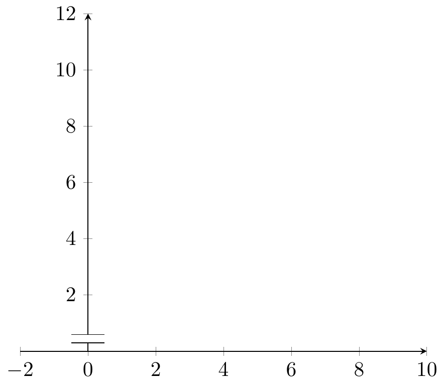
16.5.7.1.5 axis discontinuity

crunch, parallel, none

crunch

\begin{tikzpicture}
    \begin{axis}[
        axis x line = bottom,
        axis y line = center,
        xmin = -2, xmax = 10,
        ymin =  0, ymax = 12,
        axis y discontinuity = crunch,
    ]
        % empty
    \end{axis}
\end{tikzpicture}

Fig. 16.95: PGFplots: axis/axes range

parallel

\begin{tikzpicture}
    \begin{axis}[
        axis x line = bottom,
        axis y line = center,
        xmin = -2, xmax = 10,
        ymin =  0, ymax = 12,
        axis y discontinuity = parallel,
    ]
        % empty
    \end{axis}
\end{tikzpicture}

Fig. 16.96: PGFplots: axis/axes range

16.5.7.1.6 tick

tick pos ticklabel pos

\begin{tikzpicture}
    \begin{axis}[
        xtick pos = upper,
        yticklabel pos = upper,
    ]
        % empty
    \end{axis}
\end{tikzpicture}

Fig. 16.97: PGFplots: axis/axes range

tick distance

tick align: inside, center, outside

\begin{tikzpicture}
    \begin{axis}[
        axis lines=center,
        xmin=-1,xmax=3,
        ymin=-3,ymax=3,
        xtick distance=.8,
        ytick distance=1.1,
        tick align=inside,
    ]
        % empty
    \end{axis}
\end{tikzpicture}

Fig. 16.98: PGFplots: axis/axes range

minor tick num

\begin{tikzpicture}
    \begin{axis}[
        axis y line=none,axis x line=center,
        ymin=0,ymax=0,xmin=-3,xmax=3,
        xtick distance=2,tick align=inside,
        minor tick num=2,
    ]
        % empty
    \end{axis}
\end{tikzpicture}

Fig. 16.99: PGFplots: axis/axes range

xtick=\empty|data|{<coordinates>}

\begin{tikzpicture}
    \begin{axis}[
        axis y line=none,axis x line=center,
        ymin=0,ymax=0,xmin=-3,xmax=3,
        xtick={-2.5,0,1},minor xtick={1/3,2/3},
        tick align=inside,
        ]
        % empty
    \end{axis}
\end{tikzpicture}

Fig. 16.100: PGFplots: axis/axes range

extra x ticks={<coordinates>}

\begin{tikzpicture}
    \begin{axis}[
        axis y line=none,axis x line=center,
        ymin=0,ymax=0,xmin=-2.3,xmax=4.9,
        xtick distance=2,minor tick num=1,
        extra x ticks={e,pi},
        extra x tick labels={$e$,$\pi$},
        tick align=inside,
    ]
        % empty
    \end{axis}
\end{tikzpicture}

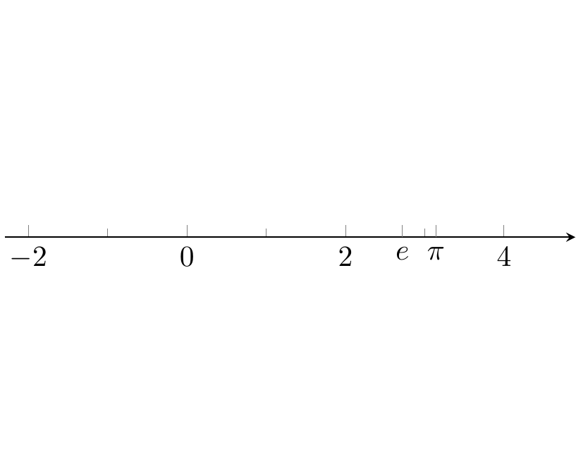
Fig. 16.101: PGFplots: axis/axes range

ticklabels={<labels>} extra x tick labels={<labels>}

hide obscured x ticks = false for origin x tick label

\begin{tikzpicture}
    \begin{axis}[
        axis y line=none,axis x line=center,
        ymin=0,ymax=0,xmin=-2.3*pi,xmax=2.3*pi,
        xtick distance=pi,
        xticklabels={$-2\pi$,$-\pi$,$0$,$\pi$,$2\pi$},
    ]
        % empty
    \end{axis}
\end{tikzpicture}

Fig. 16.102: PGFplots: axis/axes range

16.5.7.2 `addplot+`

What does addplot+ do exactly?

https://tex.stackexchange.com/questions/275959/what-does-addplot-do-exactly

https://tikz.dev/pgfplots/reference-addplot#\addplot+

Every \addplot directive receives a pre-defined style (line color, marker style etc) through a pre-defined cycle list that is automatically chosen depending on the index of the current \addplot instruction. If you want to add some of your styles manually (like I want red colour instead of blue, say), you can add them through options to \addplot like \addplot[<your options>]. Now the question is whether you want your own style (your options) to be appended to or replace one of these cycle lists assigned. This is decided by the + sign. If you use \addplot+ [<your options>], your style is appended to and by \addplot[<your options>] , your options will replace the assigned cycle list.

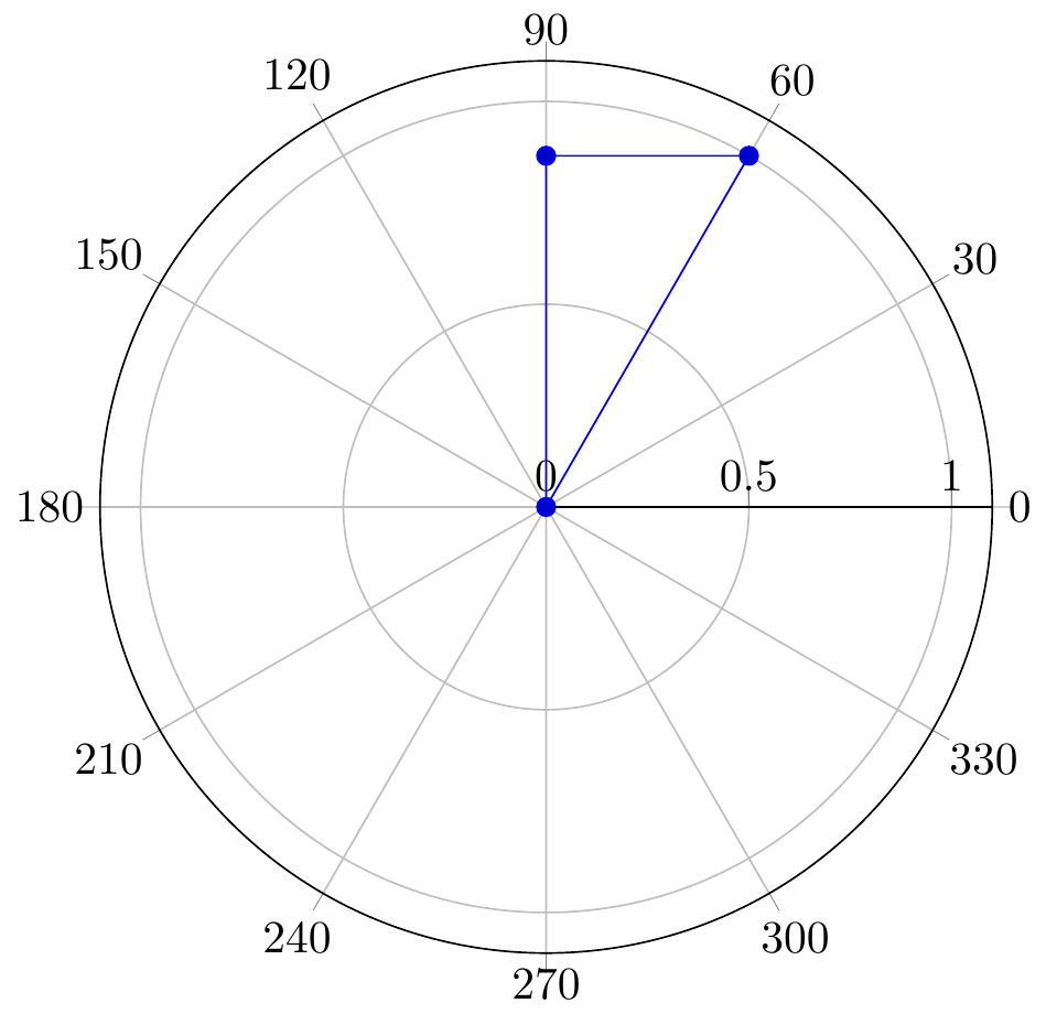
16.5.7.3 point

only marks only points without lines

zero y axis range ymin=0, ymax=0 and axis y line=none, making 1D x axis

\begin{tikzpicture}
    \begin{axis}[ 
        xlabel=$x$,
        axis y line=none,
        axis x line=center,
        tick align=inside,
        xmin=-1.5, xmax=4.9, ymin=0, ymax=0,
        xtick distance=1,
        x=1cm
        ]
        \addplot+ coordinates {(e,0)}
            node [pin=90:{$e$}] {};
        \addplot+ coordinates {(pi,0)}
            node [pin=90:{$\pi$}] {};
        \addplot+ coordinates {(-1,0)};
    \end{axis}
\end{tikzpicture}

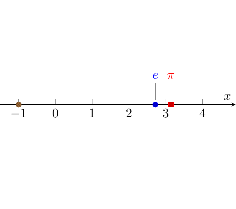
Fig. 16.103: PGFplots: 1D points with pins

\begin{tikzpicture}
    \begin{axis}[
        xlabel=$x$, ylabel=$y$,
        axis lines=center,
        tick align=inside,
        xmin=-1.5, xmax=4.9, ymin=-3.3, ymax=3.9,
        xtick distance=1, ytick distance=1,
        axis equal image
        ]
        \addplot+ [only marks] coordinates {
            (-1,-2) (pi,pi/4) (3,2) (0,0)};
        \addplot+ coordinates {(2,1)};
        \addplot+ coordinates {(3,-2)};
    \end{axis}
\end{tikzpicture}

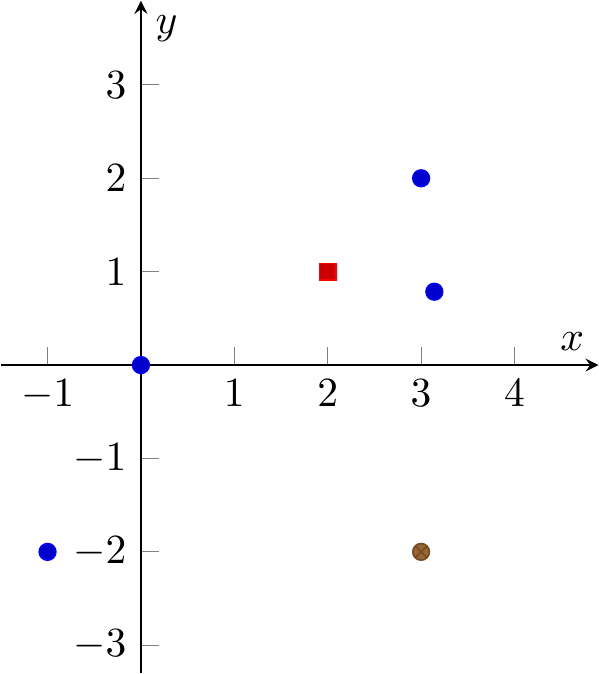
Fig. 16.104: PGFplots: 2D points

\begin{tikzpicture}
    \begin{axis}[axis equal image]
        \addplot+ [only marks]
            table [x=xdata,y=ydata] {data/func.dat};
    \end{axis}
\end{tikzpicture}

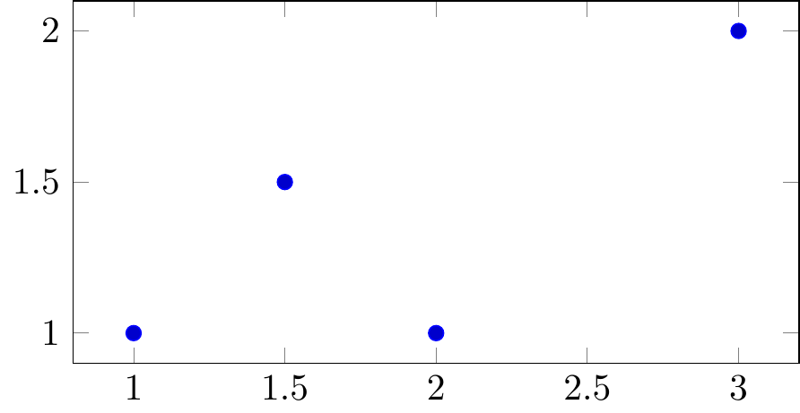
Fig. 16.105: PGFplots: data points

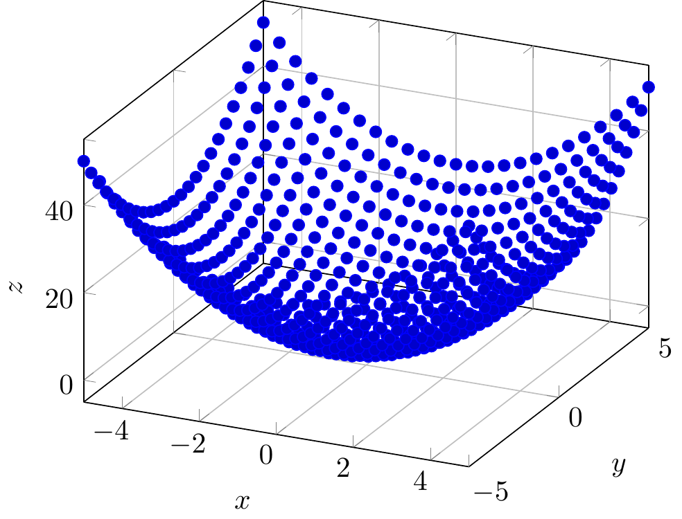
axis equal image to fix aspect ratio 1:1

\begin{tikzpicture}
    \begin{axis}[title=5 sampling points,
        xlabel=$x$,ylabel=$y$,
        axis equal image]
        \addplot+ [only marks,domain=-2:2,samples=5]
            {x^2};
    \end{axis}
\end{tikzpicture}

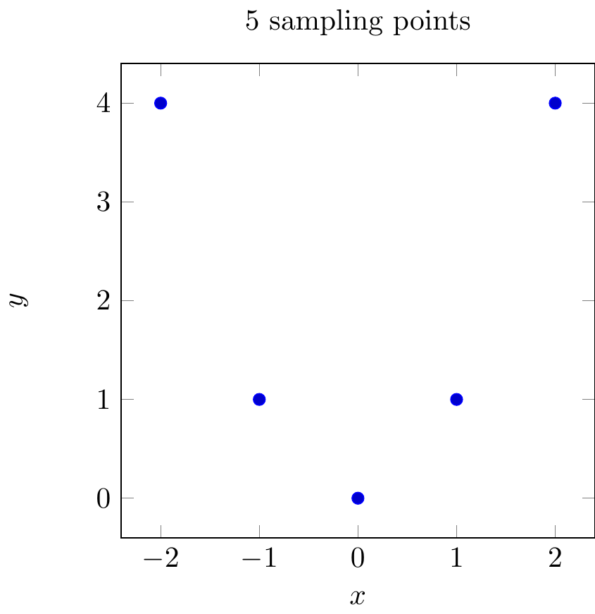
Fig. 16.106: PGFplots: function sampling 5 points

\begin{tikzpicture}
    \begin{axis}[title=55 sampling points,
        xlabel=$x$,ylabel=$y$,
        axis equal image]
        \addplot+ [only marks,domain=-2:2,samples=55]
            {x^2};
    \end{axis}
\end{tikzpicture}

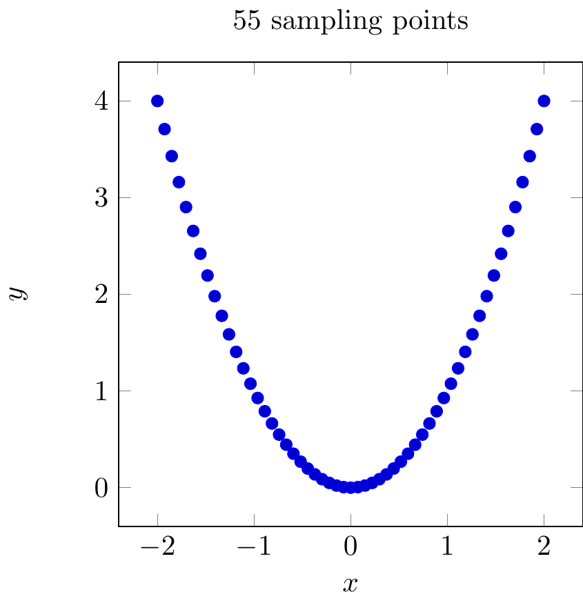
Fig. 16.107: PGFplots: function sampling 55 points

\begin{tikzpicture}
    \begin{axis}[
        trig format plots=rad,  % angle in radian
        axis equal image]
        \addplot+ [only marks,variable=t,domain=0:pi*3/2,
            samples=20] ({cos(t)},{sin(t)});
    \end{axis}
\end{tikzpicture}

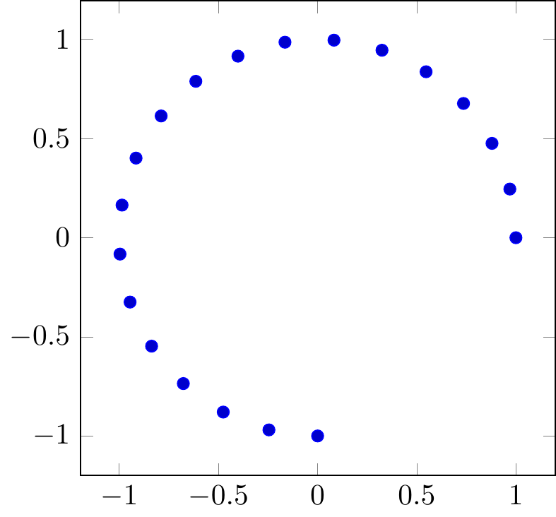
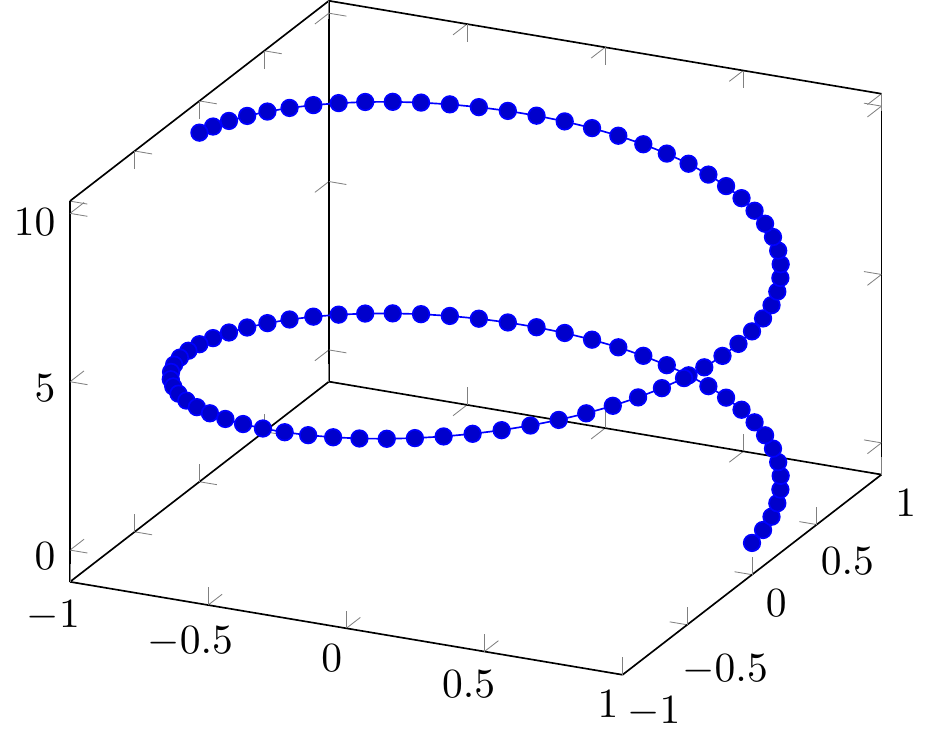
Fig. 16.108: PGFplots: parametric function sampling

\begin{tikzpicture}
    \begin{axis}[
        xlabel=$x$,ylabel=$y$,zlabel=$z$,
        axis lines=center,
        tick align=inside,
        xmin=-1.5,xmax=3.9,
        ymin=-1.5,ymax=3.9,
        zmin=-0.5,zmax=3.9,
        xtick distance=1,
        ytick distance=1,
        ztick distance=1,
        % width=10cm,
        % scale only axis,
        view={120}{30},  % perspective angle
        axis equal image,]
        \addplot3+ coordinates{(1,0,0)};
        \addplot3+ coordinates{(0,1,0)};
        \addplot3+ coordinates{(0,0,1)};
    \end{axis}
\end{tikzpicture}

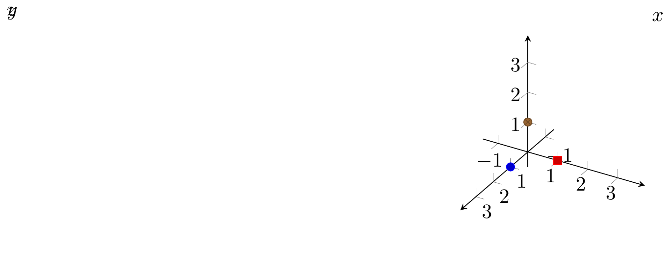
Fig. 16.109: PGFplots: 3D points

\begin{tikzpicture}
    \begin{axis}[
        xlabel=$x$,ylabel=$y$,zlabel=$z$,
        grid=major
        ]
        \addplot3+ [only marks] {x^2+y^2};
    \end{axis}
\end{tikzpicture}

Fig. 16.110: PGFplots: 3D function sampling points

16.5.7.4 line

\begin{tikzpicture}
    \begin{axis}[ytick=data]
        \addplot coordinates {
            (1,0.15) (2,0.21) (3,0.33) (4,0.4)

            (2.5,.1) (3.5,.1)
        };
    \end{axis}
\end{tikzpicture}

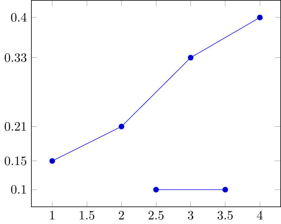
Fig. 16.111: lines connecting adjacent points

smooth to make smooth curves or lines

\begin{tikzpicture}
    \begin{axis}[ytick=data]
        \addplot+ [smooth] coordinates {
            (1,0.15) (2,0.21) (3,0.33) (4,0.4)};
    \end{axis}
\end{tikzpicture}

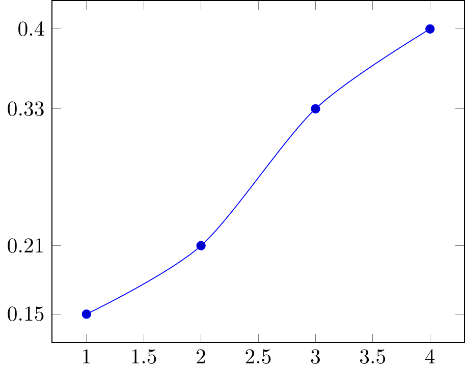
Fig. 16.112: smooth lines connecting adjacent points

no markers to make no markers or points on the curves or lines

\addlegendentry to add legends

\begin{tikzpicture}
    \begin{axis}[
        trig format plots=rad,
        xtick distance=pi/2, ytick distance=1,
        xticklabels={$-\pi$,$-\pi/2$,0,$\pi/2$,$\pi$},
        width=10cm, scale only axis,
        axis equal image]
        \addplot+ [domain=-pi:pi] {sin(x)};
        \addlegendentry{$\sin(x)$}
        \addplot+ [no markers,domain=-pi:pi,samples=100]
            {cos(x)};
        \addlegendentry{$\cos(x)$}
    \end{axis}
\end{tikzpicture}

$\sin(x)$ and $\cos(x)$

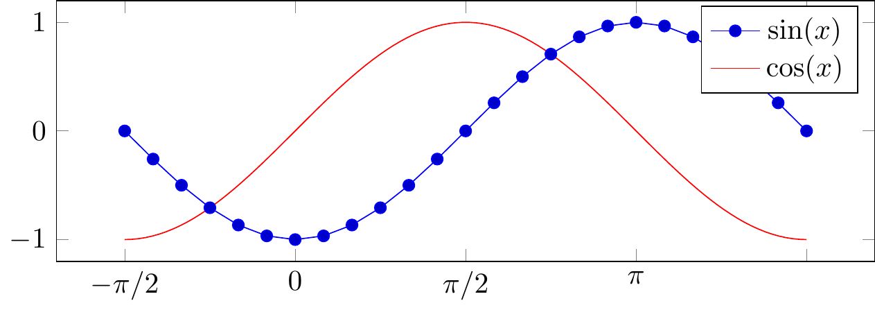
Fig. 16.113: $\sin(x)$ and $\cos(x)$

\begin{tikzpicture}
    \begin{axis}[
        trig format plots=rad,
        ymax=2.3,
        axis equal image]
        \addplot+ [no markers,
                   variable=t,
                   domain=0:2*pi,
                   samples=100] ({2*cos(t)},{sin(t)});
        \node [pin=90:$\dfrac{x^2}{4}+y^2{=}1$]
        at ({2*cos(45)},{sin(45)}) {};
    \end{axis}
\end{tikzpicture}

$\dfrac{x^2}{4}+y^2{=}1$

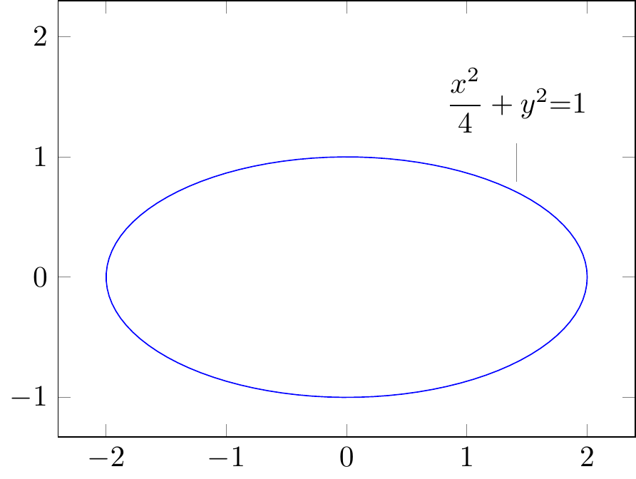
Fig. 16.114: $\dfrac{x^2}{4}+y^2{=}1$

\begin{tikzpicture}
    \begin{axis}[trig format plots=rad]
        \addplot3+ [variable=t,
                    domain=0:3*pi,
                    samples=100,
                    samples y=0]
            ({cos(t)},{sin(t)},{t});
    \end{axis}
\end{tikzpicture}

$({\cos(t)},{\sin(t)},{t})$

Fig. 16.115: $({\cos(t)},{\sin(t)},{t})$

16.5.7.5 plane

[mesh]

\begin{tikzpicture}
    \begin{axis}
        \addplot3+ [no markers, mesh] {x*y};
    \end{axis}
\end{tikzpicture}

Fig. 16.116: $f(x,y)=xy$

[surf] surface

\begin{tikzpicture}
    \begin{axis}[
        view={120}{30},
        trig format plots=rad,
        width=10cm,
        scale only axis,
        axis equal image
        ]
        \addplot3+ [no markers,
                    surf,
                    domain=0:2*pi,
                    domain y=0:pi]
            ({sin(y)*cos(x)},{sin(y)*sin(x)},{cos(y)});
    \end{axis}
\end{tikzpicture}

Fig. 16.117: $x^2+y^2+z^2=1$

16.5.7.6 polar coordinate

data cs=polar|polarrad

\begin{tikzpicture}
    \begin{axis}[
      title={$\rho=\cos 2\theta$},
      axis equal image
      ]
        \addplot+ [no markers,
                   data cs=polar,
                   domain=0:360,
                   samples=360
                   ] (\x,{cos(2*\x)});
    \end{axis}
\end{tikzpicture}

$polar coordinate $\rho=\cos 2\theta$$

Fig. 16.118: polar coordinate $\rho=\cos 2\theta$

\usepgfplotslibrary{polar} to use \begin{polaraxis}

\usepgfplotslibrary{polar}
\begin{tikzpicture}
    \begin{polaraxis}
        \addplot+ coordinates
            {(0,0) (60,1) (90,{sqrt(3)/2})} -- cycle;
    \end{polaraxis}
\end{tikzpicture}

Fig. 16.119: polar coordinate axes

https://zhuanlan.zhihu.com/p/128341873

16.5.8 Arnav Bandekar: Using pgfplots to make economic graphs in LaTeX

https://towardsdatascience.com/using-pgfplots-to-make-economic-graphs-in-latex-bcdc8e27c0eb

16.5.9 PGFplots gallery

https://pgfplots.sourceforge.net/gallery.html

\begin{tikzpicture}
\begin{axis}[
    xmin=-3,   xmax=3,
    ymin=-3,   ymax=3,
    extra x ticks={-1,1},
    extra y ticks={-2,2},
    extra tick style={grid=major},
]
    \draw[red] \pgfextra{
      \pgfpathellipse{\pgfplotspointaxisxy{0}{0}}
        {\pgfplotspointaxisdirectionxy{1}{0}}
        {\pgfplotspointaxisdirectionxy{0}{2}}
      % see also the documentation of 
      % 'axis direction cs' which
      % allows a simpler way to draw this ellipse
    };
    \draw[blue] \pgfextra{
      \pgfpathellipse{\pgfplotspointaxisxy{0}{0}}
        {\pgfplotspointaxisdirectionxy{1}{1}}
        {\pgfplotspointaxisdirectionxy{0}{2}}
    };
    \addplot [only marks,mark=*] coordinates { (0,0) };
\end{axis}
\end{tikzpicture}

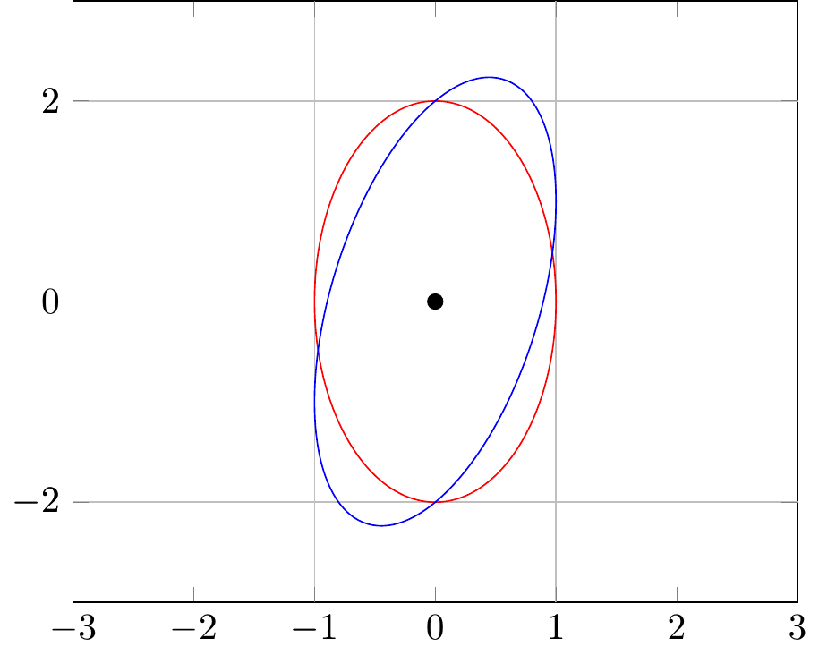
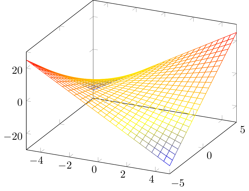
Fig. 16.120: declare function

16.6 TikZplotLib / tikzplotlib

Python^[15]

library(reticulate)

## Warning: package 'reticulate' was built under R version 4.2.3

# virtualenv_list()
# virtualenv_python()
# use_virtualenv("r-reticulate")

# conda_list()
use_condaenv(condaenv = 'sandbox-3.9')

## install TikZplotLib
# virtualenv_install("r-reticulate", "tikzplotlib")

## import TikZplotLib (it will be automatically discovered in "r-reticulate")
tikzplotlib <- import("tikzplotlib")

Error: ImportError: cannot import name 'common_texification' from 'matplotlib.backends.backend_pgf' (D:\Users\115381\Documents\.virtualenvs\r-reticulate\lib\site-packages\matplotlib\backends\backend_pgf.py)

https://github.com/NixOS/nixpkgs/issues/289305

The “solution” is to use matplotlib 3.6, but I guess in nixpkgs a single version is used at a time. The last working upgrade is from 0911608 I guess (I tried using virtualenv + pip + nix-ld + export LD_LIBRARY_PATH=“$LD_LIBRARY_PATH:$NIX_LD_LIBRARY_PATH”)

https://stackoverflow.com/questions/60882638/install-a-particular-version-of-python-package-in-a-virtualenv-created-with-reti

#reticulate::virtualenv_install(packages = c("matplotlib==3.6.0"))

reticulate::conda_list()

##                 name                                            python
## 1               base                          D:\\Anaconda3/python.exe
## 2           fiftyone          D:\\Anaconda3\\envs\\fiftyone/python.exe
## 3              keras             D:\\Anaconda3\\envs\\keras/python.exe
## 4            labelme           D:\\Anaconda3\\envs\\labelme/python.exe
## 5              manim             D:\\Anaconda3\\envs\\manim/python.exe
## 6             mmyolo            D:\\Anaconda3\\envs\\mmyolo/python.exe
## 7       r-reticulate      D:\\Anaconda3\\envs\\r-reticulate/python.exe
## 8  rsconnect-jupyter D:\\Anaconda3\\envs\\rsconnect-jupyter/python.exe
## 9            sandbox           D:\\Anaconda3\\envs\\sandbox/python.exe
## 10       sandbox-3.9       D:\\Anaconda3\\envs\\sandbox-3.9/python.exe

reticulate::use_condaenv(condaenv = 'sandbox-3.9')

import matplotlib.pyplot as plt

plt.plot([0, 2, 1, 4])
plt.show()

import tikzplotlib

# tikzplotlib.save("test.tex")
tikzplotlib.get_tikz_code()

## '% This file was created with tikzplotlib v0.10.1.\n\\begin{tikzpicture}\n\n\\end{tikzpicture}\n'

import matplotlib.pyplot as plt

plt.close()

import matplotlib.pyplot as plt
import numpy as np

plt.style.use("ggplot")

t = np.arange(0.0, 2.0, 0.1)
s = np.sin(2 * np.pi * t)
s2 = np.cos(2 * np.pi * t)
plt.plot(t, s, "o-", lw=4.1)
plt.plot(t, s2, "o-", lw=4.1)
plt.xlabel("time (s)")
plt.ylabel("Voltage (mV)")
plt.title("Simple plot $\\frac{\\alpha}{2}$")
plt.grid(True)
plt.show()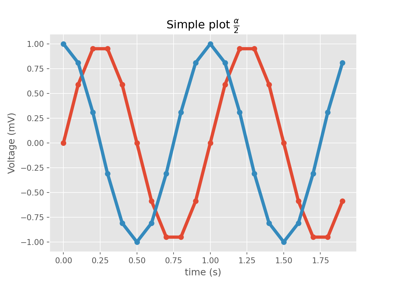

import tikzplotlib

# tikzplotlib.save("test.tex")
tikzplotlib.get_tikz_code()

## '% This file was created with tikzplotlib v0.10.1.\n\\begin{tikzpicture}\n\n\\end{tikzpicture}\n'

16.7 animation

https://zhuanlan.zhihu.com/p/338402487