Chapter 35: design of experiment
experimental design = experiment design = design of experiments = DoE
9 p.72
question-design-analysis loop
35.2 terminology
- population
- sample
- subsample
- sample
- unit
- replication (9 p.76): an independent observation of the treatment (10 p.74)
- treatment replication: experimental-unit-to-experimental-unit variation
- measurement replication = subsample: measurement-to-measurement variation
- replicate
- experimental replicate
- biological replicate
- technical replicate
10 p.73
\(Y_{\scriptscriptstyle{ij}}\): the response observed from the \(j\)th experimental unit assigned to the \(i\)th treatment
\(\mu_{\scriptscriptstyle{i}}\): the mean response to the \(i\)th treatment
\(\mathcal{E}_{\scriptscriptstyle{ij}}\): the noise from other possible natural variation or nonrandom and random error
\[ Y_{{\scriptscriptstyle i}{\scriptscriptstyle j}}=\mu_{{\scriptscriptstyle i}}+\mathcal{E}_{{\scriptscriptstyle i}{\scriptscriptstyle j}},\begin{cases} i\in\mathbb{N}\cap\left[1,n_{{\scriptscriptstyle i}}\right] & \mathbb{N}\ni n_{{\scriptscriptstyle i}}\text{ treatments}\\ j\in\mathbb{N}\cap\left[1,n_{{\scriptscriptstyle j}}\right] & \mathbb{N}\ni n_{{\scriptscriptstyle j}}\text{ experimental units per treatment} \end{cases} \]
Each treatment has \(n_{j}\) experimental units, so there are totally \(n_{i}n_{j}\) experimental units.
If experimental units cannot be homogeneous, we can try to
- stratify them
- group them, and measure group to group variation
- block them
here \(n_{j}\) blocks each with \(n_{i}\) experimental units where each treatment occurs once in each block
\[ \begin{aligned} Y_{{\scriptscriptstyle i}{\scriptscriptstyle j}}= & \mu_{{\scriptscriptstyle i}}+\mathcal{E}_{{\scriptscriptstyle i}{\scriptscriptstyle j}}\\ = & \mu_{{\scriptscriptstyle i}}+b_{{\scriptscriptstyle j}}+\mathcal{E}_{{\scriptscriptstyle i}{\scriptscriptstyle j}}^{*},\begin{cases} i\in\mathbb{N}\cap\left[1,n_{{\scriptscriptstyle i}}\right] & \mathbb{N}\ni n_{{\scriptscriptstyle i}}\text{ experimental units per block}\\ j\in\mathbb{N}\cap\left[1,n_{{\scriptscriptstyle j}}\right] & \mathbb{N}\ni n_{{\scriptscriptstyle j}}\text{ blocks} \end{cases} \end{aligned} \]
where
\[ \mathcal{E}_{{\scriptscriptstyle i}{\scriptscriptstyle j}}=b_{{\scriptscriptstyle j}}+\mathcal{E}_{{\scriptscriptstyle i}{\scriptscriptstyle j}}^{*} \]
i.e. the variation between groups or blocks of experimental units has been identified and isolated from \(\mathcal{E}_{ij}^{*}\), which represents the variability of experimental units within a block. By isolating the block effect from the experimental units, the within-block variation can be used to compare treatment effects, which involves computing the estimated standard errors of contrasts of the treatments.
\[ \begin{aligned} Y_{{\scriptscriptstyle i}{\scriptscriptstyle j}}-Y_{{\scriptscriptstyle i^{\prime}}{\scriptscriptstyle j}}= & \left(\mu_{{\scriptscriptstyle i}}+b_{{\scriptscriptstyle j}}+\mathcal{E}_{{\scriptscriptstyle i}{\scriptscriptstyle j}}^{*}\right)\\ - & \left(\mu_{{\scriptscriptstyle i^{\prime}}}+b_{{\scriptscriptstyle j}}+\mathcal{E}_{{\scriptscriptstyle i^{\prime}}{\scriptscriptstyle j}}^{*}\right)\\ = & \left(\mu_{{\scriptscriptstyle i}}-\mu_{{\scriptscriptstyle i^{\prime}}}\right)+\left(\mathcal{E}_{{\scriptscriptstyle i}{\scriptscriptstyle j}}^{*}-\mathcal{E}_{{\scriptscriptstyle i^{\prime}}{\scriptscriptstyle j}}^{*}\right) \end{aligned} \]
which does not depend on the block effect \(b_{j}\) or free of block effects. The result of this difference is that the variance of the difference of two treatment responses within a block depends on the within-block variation among the experimental units and not the between-block variation.
35.2.1 replication vs. subsample
It is very important to distinguish between a subsample and a replication since the error variance estimated from between subsamples is in general considerably smaller than the error variance estimated from replications or between experimental units. (10 p.77)
35.2.3 replication, replicate
35.2.3.1 technical replicate, biological replicate
https://www.youtube.com/watch?v=c_cpl5YsBV8
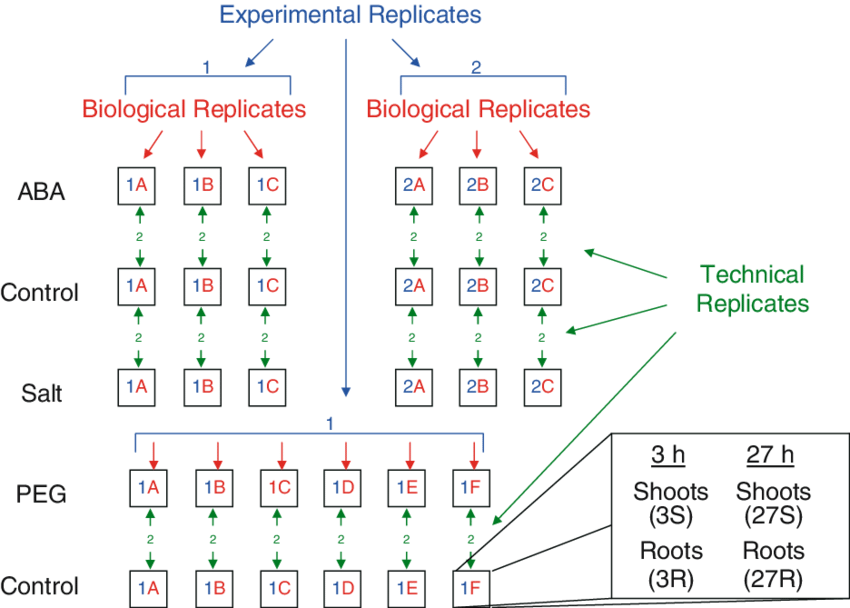
Fig. 24.1: experimental, biological, technical replicates ( 11)
35.2.4 Latin square design
LSD = Latin square design
6 p.505~507
https://tex.stackexchange.com/questions/501671/how-to-get-math-mode-curly-braces-in-tikz
\\usepackage{pgfplots} in engine.opts=list(extra.preamble=c("\\usepackage{pgfplots}"))
\usetikzlibrary{decorations}
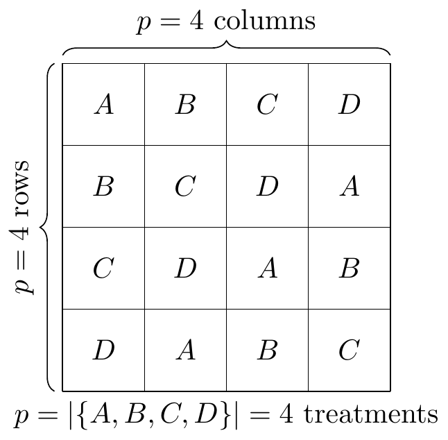
Fig. 30.2: Latin square example
\[ Y_{{\scriptscriptstyle ijk}}=\mu+\alpha_{{\scriptscriptstyle i}}+\beta_{{\scriptscriptstyle j}}+\gamma_{{\scriptscriptstyle k}}+\mathcal{E}_{{\scriptscriptstyle ijk}},\begin{cases} i\in\mathbb{N}\cap\left[1,p\right] & \mathbb{N}\ni p\text{ treatments}\\ j\in\mathbb{N}\cap\left[1,p\right] & \mathbb{N}\ni p\text{ rows}\\ k\in\mathbb{N}\cap\left[1,p\right] & \mathbb{N}\ni p\text{ columns} \end{cases} \]
\[ \mathcal{E}_{{\scriptscriptstyle ijk}}\overset{\text{i.i.d.}}{\sim}\mathrm{n}\left(0,\sigma^{2}\right) \]
\(\rho_{{\scriptscriptstyle i}}\): \(i\)th row
\(\kappa_{{\scriptscriptstyle j}}\): \(j\)th column
\(\tau_{{\scriptscriptstyle k}}\): \(k\)th treatment
\[ \begin{aligned} Y_{{\scriptscriptstyle ijk}}= & \mu+\alpha_{{\scriptscriptstyle i}}+\beta_{{\scriptscriptstyle j}}+\gamma_{{\scriptscriptstyle k}}+\mathcal{E}_{{\scriptscriptstyle ijk}},\begin{cases} i\in\mathbb{N}\cap\left[1,p\right] & \mathbb{N}\ni p\text{ treatments}\\ j\in\mathbb{N}\cap\left[1,p\right] & \mathbb{N}\ni p\text{ rows}\\ k\in\mathbb{N}\cap\left[1,p\right] & \mathbb{N}\ni p\text{ columns} \end{cases}\\ = & \mu+\rho_{{\scriptscriptstyle i}}+\kappa_{{\scriptscriptstyle j}}+\tau_{{\scriptscriptstyle k}}+\mathcal{E}_{{\scriptscriptstyle ijk}},\begin{cases} i\in\mathbb{N}\cap\left[1,p\right] & \mathbb{N}\ni p\text{ rows}\\ j\in\mathbb{N}\cap\left[1,p\right] & \mathbb{N}\ni p\text{ columns}\\ k\in\mathbb{N}\cap\left[1,p\right] & \mathbb{N}\ni p\text{ treatments} \end{cases} \end{aligned} \]
35.2.5 model assumption and experimental unit, measurement/observational unit
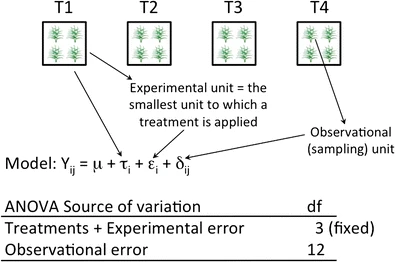
Fig. 17.1: model assumption and experimental unit 1 ( 12 fig.1)
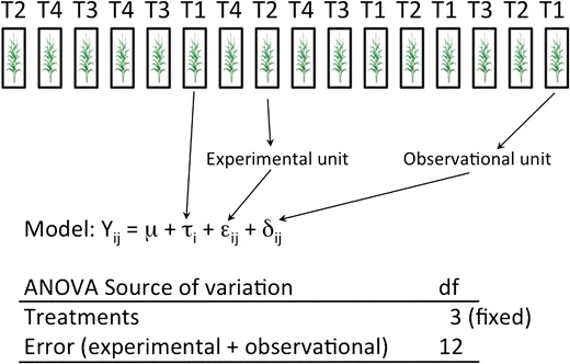
Fig. 17.2: model assumption and experimental unit 2 ( 12 fig.2)
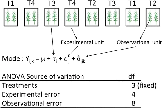
Fig. 24.2: model assumption and experimental unit 3 ( 12 fig.3)
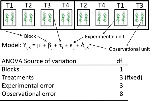
Fig. 16.1: model assumption and experimental unit 4 ( 12 fig.4)
\[ Y_{{\scriptscriptstyle ijk}}=\mu+\tau_{{\scriptscriptstyle i}}+\beta_{{\scriptscriptstyle j}}+\epsilon_{{\scriptscriptstyle ij}}+\varDelta_{{\scriptscriptstyle ijk}} \]
35.3 experiment structure
35.3.1 treatment structure
10 p.77
- 1-way treatment structure
- 2-way treatment structure
- factorial arrangement treatment structure
- fractional factorial arrangement treatment structure
- factorial arrangement with one or more controls
35.3.2 design structure
10 p.77
- CRD = completely randomized design
- RCBD = randomized complete block design
- ? why not called CRBD = completely randomized block design
- LSD = Latin square design[35.2.4]
- IBD = incomplete block design
- BIBD = balanced IBD
- various combinations and generalizations
35.4 approach to experimentation
9 p.75
- approach to experimentation
- best-guess approach
- one-factor-at-a-time approach = OFAT
- factorial approach
35.7 protocol
9 p.95
- study objective
- study endpoint
- primary endpoint
- secondary endpoint(s)
- experimental unit(s)
- treatment structure[35.3.1]
- design structure[35.3.2]
- potential confounder(s)
- randomization
- blinding
- chance reduction
- sample size estimation[35.5]
- data collection
- data management system
- statistical analysis plan[35.6]
- DSMB / DSMC = data and safety monitoring board / committee