6.2 time ordering 2

$$\langle\phi_0(t_f)^3 \phi_1\phi_0^3(t) \phi_1(0) \rangle \to \langle 0|\phi_0|3\phi_0 \rangle \langle 3\phi_0| \phi_1 \phi_0^3 | \phi_1\rangle \langle \phi_1|\phi_1|0 \rangle e^{-E_{3\phi_0}(t_f)+(E_{3\phi_0}-E_{\phi_1})t } \\+ \langle \phi_0|\phi_0^3|2\phi_0 \rangle \langle 2\phi_0| \phi_1 \phi_0^3 |2 \phi_0\phi_1\rangle \langle \phi_1|\phi_1|\phi_0 \rangle e^{\color{red}{-E_{2\phi_0}(t_f)}-\color{blue}{E_{\phi_0}(T-t_f)}+\color{blue}{(E_{2\phi_0}-E_{\phi_0\phi_1})t} } \\+ \langle 2\phi_0|\phi_0^3|\phi_0 \rangle \langle \phi_0| \phi_1 \phi_0^3 | 2\phi_0\phi_1\rangle \langle 2\phi_0\phi_1|\phi_1|2\phi_0 \rangle e^{\color{red}{-E_{\phi_0}(t_f)}-\color{blue}{E_{2\phi_0}(T-t_f)}+\color{blue}{(E_{\phi_0}-E_{2\phi_0\phi_1})t} }\,.$$ suppressed, enhanced. Since $T>t_f$ the overall exponent in $T$ and $t_f$ gives an overall suppressing factor for the second and third term. If the operator $\phi^2$ has a $v.e.v$ then $\langle \phi_0|\phi^3|0\rangle \neq0$ and so there are these two more contribution $$\langle 0|\phi_0^3|\phi_0 \rangle \langle \phi_0| \phi_1 \phi_0^3 |\phi_1\rangle \langle \phi_1|\phi_1|\rangle e^{-E_{\phi_0}t_f+E_{\phi_0}t-E_{\phi_1}t} \\ +\langle \phi_0|\phi_0^3| 0\rangle \langle 0| \phi_1 \phi_0^3 |\phi_1\rangle \langle \phi_1|\phi_1|\phi_0\rangle e^{-E_{\phi_0}T+E_{\phi_0}t_f -E_{\phi_1\phi_0}t}$$

Below a plot of the different contribution assuming all the amplitude equal to 1

e1<-c()
e2<-c()
e3<-c()
e4<-c()
e5<-c()


T<-48
L<-30
tf<-16
#read the energies
dir<-"../out"
file=sprintf("%s/G2t_T%d_L%d_msq0-4.900000_msq1-4.650000_l02.500000_l12.500000_mu5.000000_g0.000000_rep0_output",dir,T,L)

mt<-read_df(file)
all_obs<- get_all_corr(mt)
E3_0=get_energy("E3_0",all_obs,mt)[1]
E1_1=get_energy("E1_1",all_obs,mt)[1]
E2_0=get_energy("E2_0",all_obs,mt)[1]
E1_0=get_energy("E1_0",all_obs,mt)[1]
E2_01=get_energy("E2_01",all_obs,mt)[1]
cat("$E_{3\\phi_0}$=",E3_0,"\n\n" )

$E_{3\phi_0}$= 0.426661

cat("$E_{1\\phi_1}$=",E1_1,"\n\n" )

$E_{1\phi_1}$= 0.4467881

cat("$E_{2\\phi_0}$=",E2_0,"\n\n" )

$E_{2\phi_0}$= 0.2604283

cat("$E_{1\\phi_0}$=",E1_0,"\n\n" )

$E_{1\phi_0}$= 0.1283262

t<-c(0:480)/100
e1<-c(e1, exp(-E3_0*tf+(E3_0-E1_1)*t ) )
e2<-c(e2, exp(-E2_0*tf-E1_0*(T-tf)+ (E2_0-(E1_0+E1_1) )*t ) )
e3<-c(e3, exp(-E1_0*tf-E2_0*(T-tf)+ (E1_0-(E2_0+E1_1))*t ) )
e4<-c(e4, exp(-E1_0*tf + E1_0*t- E1_0*t ) )
e5<-c(e5, exp(-E1_0*T + (E1_0)*tf- (E1_0+E1_1)*t   ) )

gg<-ggplot()+geom_line(aes(x=t,y=log(e1), color="1"))+theme_bw()
gg<-   gg   +geom_line(aes(x=t,y=log(e2), color="2"))
gg<-   gg   +geom_line(aes(x=t,y=log(e3), color="3"))
gg<-   gg   +geom_line(aes(x=t,y=log(e4), color="4"))
gg<-   gg   +geom_line(aes(x=t,y=log(e5), color="5"))
gg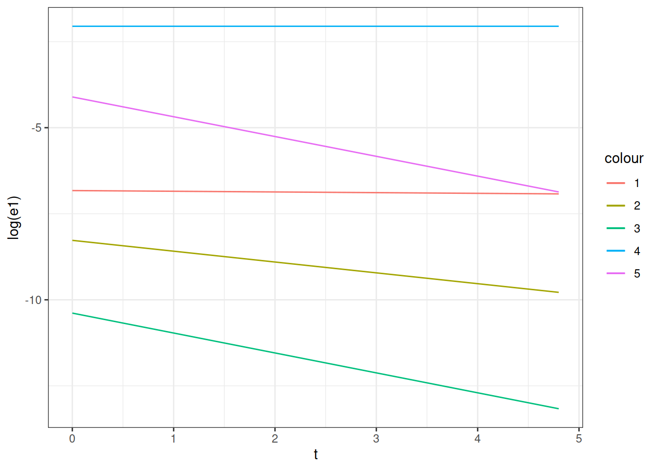

6.2.1 Fittint the contribution 1,4,5

6.2.1.1 ../out/G2t_T48_L30_msq0-4.900000_msq1-4.650000_l02.500000_l12.500000_mu5.000000_g0.000000_rep0_output

me_3pik_T_2(L30T48) = -0.1(0.2)e-13 10.6(0.4)e-12 10.0(0.6)e-12 $\chi^2/dof=$ 0.062786

me_3pik_t10(L30T48) = 2.3(0.2)e-15 10.3(0.2)e-12 1.3(0.9)e-11 $\chi^2/dof=$ 0.16098

me_3pik_t12(L30T48) = 2.3(0.3)e-15 10.2(0.2)e-12 1.2(0.6)e-11 $\chi^2/dof=$ 0.15501

me_3pik_t16(L30T48) = 1.3(0.9)e-15 10.5(0.2)e-12 0.8(0.2)e-11 $\chi^2/dof=$ 0.15171

6.2.1.2 ../out/G2t_T96_L30_msq0-4.900000_msq1-4.650000_l02.500000_l12.500000_mu5.000000_g0.000000_rep0_output

me_3pik_T_2(L30T96) = -0.1(0.1)e-9 1.6(0.6)e-11 0.6(0.7)e-11 $\chi^2/dof=$ 0.10744

me_3pik_t10(L30T96) = 2.1(0.1)e-15 10.3(0.1)e-12 -0.0(0.3)e-8 $\chi^2/dof=$ 0.11626

me_3pik_t12(L30T96) = 2.0(0.2)e-15 10.3(0.1)e-12 -0.0(0.2)e-8 $\chi^2/dof=$ 0.10779

me_3pik_t16(L30T96) = 2.3(0.6)e-15 10.1(0.1)e-12 0.6(0.6)e-9 $\chi^2/dof=$ 0.30898