4.3 Continuous random variables: Probability density functions

The continuous analog of a pmf is a probability density function. However, while pmfs and pdfs play analogous roles, they are different in one fundamental way; namely, a pmf outputs probabilities directly, while a pdf does not. We have seen that a pmf of a discrete random variable can be summed to find probabilities of related events. We will see now that a pdf of a continuous random variable must be integrated to find probabilities of related events.

In Section 3.6 we introduced histograms to summarize simulated values of a continuous random variable. In a histogram the variable axis is chopped into intervals of equal width, and the other axis is on the density scale, so that the area of each bar represents the relative frequency of values that lie in the interval.

We have seen examples (e,g., Figures 3.10, 3.11) where the shape of the histogram can be approximated by a smooth curve. This curve represents an idealized model of what the histogram would look like if infinitely many values were simulated and the histogram bins were infinitesimally small.

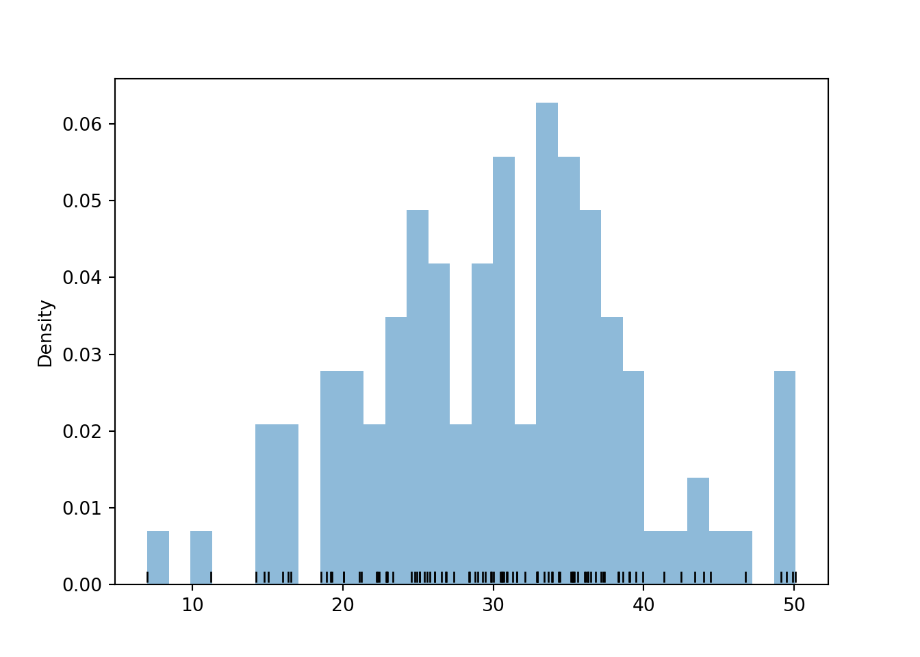
Consider Figure 3.11 which summarizes 10000 simulated values of the random variable $X = - \log(1 - U)$ where $U$ has a Uniform(0, 1) distribution. Imagine that we

• keep simulating more and more values, and
• make the histogram bin widths smaller and smaller.

Then the “chunky” histogram would get “smoother”. The following plot summarizes the results of 100,000 simulated values of $X$ in a histogram with 1000 bins, each of width on the order of 0.01. The command Exponential(1).plot() overlays the smooth curve modeling the theoretical shape of the distribution of $X$ (called the “Exponential(1)” distribution). This curve is an example of a pdf.

U = RV(Uniform(0, 1))

X = -log(1 - U)

X.sim(100000).plot(bins=1000)
Exponential(1).plot() # overlays the smooth curve
plt.show()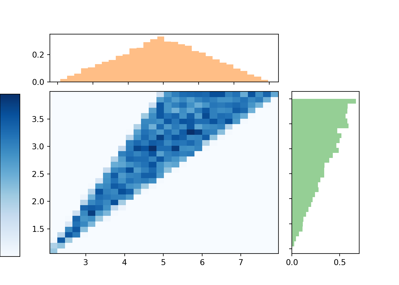

A pdf represents “relative likelihood” as a function of possible values of the random variable. Just as area represents relative frequency in a histogram, area under a pdf represents probability.

Definition 4.3 The probability density function (pdf) (a.k.a. density) of a continuous RV $X$, defined on a probability space with probability measure $\textrm{P}$, is a function $f_X:\mathbb{R}\mapsto[0,\infty)$ which satisfies $$\begin{align*} \textrm{P}(a \le X \le b) & =\int_a^b f_X(x) dx, \qquad \text{for all } -\infty \le a \le b \le \infty \end{align*}$$

For a continuous random variable $X$ with pdf $f_X$, the probability that $X$ takes a value in the interval $[a, b]$ is the area under the pdf over the region $[a,b]$.

Example 4.11 Recall Example 2.38. Regina and Cady plan to meet for lunch between noon and 1 but they are not sure of their arrival times. We’ll consider only Regina’s arrival time for now. (We’ll get back to Cady soon.) Assume that Regina arrives at a time chosen uniformly at random between noon and 1. We can model Regina’s arrival with the sample space $[0, 1]$ and a uniform probability measure. Let $X$ be Regina’s arrival time in $[0, 1]$.

1. Sketch a plot of the pdf of $X$.
2. Donny Dont says that the pdf is $f_X(x) = 1$. Do you agree? If not, specify the pdf of $X$.
3. Use the pdf to find the probability that Regina arrives before 12:15.
4. Use the pdf to find the probability that Regina arrives after 12:45.
5. Use the pdf to find the probability that Regina arrives between 12:15 and 12:45.
6. Use the pdf to find the probability that Regina arrives between 12:15:00 and 12:16:00.
7. Use the pdf to find the probability that Regina arrives between 12:15:00 and 12:15:01.
8. Use the pdf to find the probability that Regina arrives at the exact time 12:15:00 (with infinite precision).

Solution. to Example 4.11

Show/hide solution

1. We expect the height of the pdf to be constant between 0 and 1, both because her arrival time is uniform over the interval so no one value should be more likely than another, and because when we simulated values the histogram bars had roughly constant height. See the plot below.
2. We need the area under the curve over the interval $[0, 1]$ to be 1, representing 100% probability. If the height of the density is $c$, a constant, then the area under the curve is the area of a rectangle with base 1 (length of the interval $[0, 1]$) and height $c$. So $c$ needs to be 1 for the total area to be 1.
   However, Donny Don’t hasn’t specified the possible values. It’s possible that someone who sees Donny’s expression would think that $f_X(2.5)=1$. But the pdf is only 1 over the range $[0, 1]$; it is 0 outside of this range. A more precise expression is $$f_X(x) = \begin{cases} 1, & 0\le x \le 1,\\ 0, & \text{otherwise.} \end{cases}$$ You don’t necessarily always need to write “0 otherwise”, but do always provide the possible values.
3. Integrate the pdf over the range $[0, 0.25]$. Since the pdf has constant height, areas under the curve just correspond to areas of rectangles. $$\textrm{P}(X \le 0.25) = \int_0^{0.25} 1 dx = x\Big|_{x = 0}^{x = 0.25} = 0.25$$
4. Integrate the pdf over the range $[0.75, 1]$.
   $$\textrm{P}(X \ge 0.75) = \int_{0.75}^1 1 dx = x\Big|_{x = 0.75}^{x = 1} = 1-0.75 = 0.25$$
5. We could use the previous parts, but we’ll intergrate the pdf over the range $[0.25, 0.75]$. $$\textrm{P}(0.25 \le X \le 0.75) = \int_{0.25}^{0.75} 1 dx = x\Big|_{x = 0.25}^{x = 0.75} = 0.75 -0.25 = 0.5$$ .
6. Integrate the pdf over the range $[0.25, 0.25 + 1/60]$.
   $$\textrm{P}(0.25 \le X \le 0.25 + 1/60) = 1/60$$
7. Integrate the pdf over the range $[0.25, 0.25 + 1/3600]$.
   $$\textrm{P}(0.25 \le X \le 0.25 + 1/3600) = 1/3600$$
8. $\textrm{P}(X = 0.25) = 0$. Integrate the pdf over the range $[0.25, 0.25]$. The region under the curve at this single point corresponds to a line segment which has 0 area. $$\textrm{P}(X = 0.25) = \int_{0.25}^{0.25} 1 dx = 0$$

Uniform(0, 1).plot()

plt.fill_between([0.25, 0.75], 1, 0, color='orange', alpha=0.2) # shade the region

plt.show()

Figure 4.4: The pdf of a Uniform(0, 1) distribution. The blue line represents the pdf. The shaded orange region represents the probability of the interval [0.25, 0.75].

A pdf assigns zero probability to intervals where the density is 0. A pdf is usually defined for all real values, but is often nonzero only for some subset of values, the possible values of the random variable. We often write the pdf as $$f_X(x) = \begin{cases} \text{some function of $x$}, & \text{possible values of $x$}\\ 0, & \text{otherwise.} \end{cases}$$

The axioms of probability imply that a valid pdf must satisfy $$\begin{align*} f_X(x) & \ge 0 \qquad \text{for all } x,\\ \int_{-\infty}^\infty f_X(x) dx & = 1 \end{align*}$$

The total area under the pdf must be 1 to represent 100% probability. Given a specific pdf, the generic bounds $(-\infty, \infty)$ in the above integral should be replaced by the range of possible values, that is, those values for which $f_X(x)>0$.

Example 4.12 Suppose that SAT Math scores follow a Uniform(200, 800) distribution. Let $U$ be the Math score for a randomly selected student.

1. Identify $f_U$, the pdf of $U$.
2. Donny Dont says that the probability that $U$ is 500 is 1/600. Do you agree? If not, explain why not.
3. While modeling SAT Math score as a continuous random variable might be mathematically convenient, it’s not entirely practical. Suppose that the range of values $[495, 505)$ corresponds to students who actually score 500. Find $\textrm{P}(495 \le X < 500)$.

Solution. to Example 4.12

Show/hide solution

1. The density still has constant height. But now the height has to be 1/600 so that the total area under the pdf over the range of possible values $[200, 800]$ is 1. So $f_U(u) = \frac{1}{600}, 200<u<800$ (and $f_U(u)=0$ otherwise).
2. It is true that $f_U(500)=1/600$. However, $f_U(500)$ is NOT $\textrm{P}(U=500)$. The density (height) at a particular point is not the probability of anything. Probabilities are determined by integrating the density. The “area” under the curve for the region $[500,500]$ is just a line segment, which has area 0, so $\textrm{P}(U=500)=0$. Integrating, $\int_{500}^{500}(1/600)du=0$. More on this point below.
3. $\textrm{P}(495 \le U < 505)=(505-495)(1/600) = 1/60$. The integral $\int_{495}^{505}(1/600)du$ corresponds to the area of a rectangle with base $505-495$ and height 1/600, so the area is 1/60.

The pdf of a general Uniform($a$, $b$) distribution is $$\text{Uniform($a$, $b$) pdf:} \qquad f(x) = \begin{cases} \frac{1}{b-a}, & a\le x\le b,\\ 0, & \text{otherwise.} \end{cases}$$

Plugging a value into the pdf of a continuous random variable does not provide a probability. The pdf itself does not provide probabilities directly; instead a pdf must be integrated to find probabilities.

The probability that a continuous random variable $X$ equals any particular value is 0. That is, if $X$ is continuous then $\textrm{P}(X=x)=0$ for all $x$. Therefore, for a continuous RV⁶⁵, $\textrm{P}(X\le x) = \textrm{P}(X<x)$, etc. A continuous random variable can take uncountably many distinct values. Simulating values of a continuous random variable corresponds to an idealized spinner with an infinitely precise needle which can land on any value in a continuous scale.

In the Uniform(0, 1) case, $0.500000000\ldots$ is different than $0.50000000010\ldots$ is different than $0.500000000000001\ldots$, etc. Consider the spinner in Figure 2.2. The spinner in the picture is only labeled in 100 increments of 0.01 each; when we spin, the probability that the needle lands closest to the 0.5 tick mark is 0.01. But if the spinner were labeled in increments 1000 increments of 0.001, the probability of landing closest to the 0.5 tick mark is 0.001. And with four decimal places of precision, the probability is 0.0001. And so on. The more precise we mark the axis, the smaller the probability the spinner lands closest to the 0.5 tick mark. The Uniform(0, 1) density represents what happens in the limit as the spinner becomes infinitely precise. The probability of landing closest to the 0.5 tick mark gets smaller and smaller, eventually becoming 0 in the limit.

A density is an idealized mathematical model. In practical applications, there is some acceptable degree of precision, and events like “$X$, rounded to 4 decimal places, equals 0.5” correspond to intervals that do have positive probability. For continuous random variables, it doesn’t really make sense to talk about the probability that the random value equals a particular value. However, we can consider the probability that a random variable is close to a particular value.

Example 4.13 Continuing Example 4.11, we will now we assume Regina’s arrival time in $[0, 1]$ has pdf

$$f_X(x) = \begin{cases} cx, & 0\le x \le 1,\\ 0, & \text{otherwise.} \end{cases}$$

where $c$ is an appropriate constant.

1. Sketch a plot of the pdf. What does this say about Regina’s arival time?
2. Find the value of $c$ and specify the pdf of $X$.
3. Find the probability that Regina arrives before 12:15.
4. Find the probability that Regina arrives after 12:45. How does this compare to the previous part? What does that say about Regina’s arrival time?
5. Find the probability that Regina arrives between 12:15 and 12:45.
6. Find the probability that Regina arrives between 12:15:00 and 12:15:01.
7. Find the probability that Regina arrives at the exact time 12:15:00 (with infinite precision).
8. Find the probability that Regina arrives between 12:59:00 and 1:00:00. How does this compare to the probability for 12:15:00 to 12:16:00? What does that say about Regina’s arrival time?
9. Find the probability that Regina arrives between 12:59:59 and 1:00:00. How does this compare to the probability for 12:15:00 to 12:15:01? What does that say about Regina’s arrival time?
10. Find the probability that Regina arrives at the exact time 1:00:00 (with infinite precision).

Solution. to Example 4.13

Show/hide solution

1. The density increases linearly with $r$. Regina is most likely to arrive closer to 1, and least likely to arrive close to noon (0).
2. $c=2$. The total area under the pdf must be 1. The region under the pdf is a triangle with area $(1/2)(1-0)(c)$, so $c$ must be 2 for the area to be 1. Via integration $$1 = \int_0^1 cx dx = (c/2)x^2 \Big|_{x=0}^{x=1} = c / 2$$
3. Integrate the pdf over the region $[0, 0.25]$. Since the pdf is linear, regions under the curve are triangles or trapezoids. $$\int_0^{0.25} 2x dx = x^2 \Bigg|_{x=0}^{x=0.25} = 0.25^2 = (1/2)(0.25 - 0)(2(0.25)) = 0.0625$$
4. Integrate the pdf over the region $[0.75, 1]$. $$\int_{0.75}^1 2x dx = x^2 \Bigg|_{x=0.75}^{x=1} = 1 - 0.75^2 = 0.4375$$ So Regina is 7 times more likely to arrive within 15 minutes of 1 than within 15 minutes of noon.
5. 0.5
6. Similar to the previous parts, the probability is $(0.25 + 1/60)^2 - 0.25^2 = 0.0086$. (This probability is less than what it was in the uniform case.)
7. Similar to the previous part, $(0.25 + 1/3600)^2 - 0.25^2 = 0.00014$. (This probability is less than what it was in the uniform case.)
8. The exact time 12:15:00 represents a single point the sample space, an interval of length 0. 1. The probability that Regina arrives at the exact time 12:15:00 (with infinite precision) is 0.
9. Similar to previous parts, $1^2 - (1-1/60)^2 = 0.0331$. Notice that this one minute interval around 1:00 has a probability that is about 3.85 times larger than a one minute interval around 12:15.
10. $1^2 - (1-1/3600)^2 = 0.00056$. Notice that this one second interval around 1:00 has a probability that is about 4 times higher than a one second interval around 12:15, though both probabilities are small.
11. The exact time 1:00:00 represents a single point the sample space, an interval of length 0. The probability that Regina arrives at the exact time 1:00:00 (with infinite precision) is 0.

In the previous example, we specified the general shape of the pdf, then found the constant that made the total area under the curve equal to 1. In general, a pdf is often defined only up to some multiplicative constant $c$, for example $f_X(x) = c\times(\text{some function of x})$, or $f_X(x) \propto \text{some function of x}$. The constant $c$ does not affect the shape of the distribution as a function of $x$, only the scale on the density axis. The absolute scaling on the density axis is somewhat irrelevant; it is whatever it needs to be to provide the proper area. In particular, the total area under the pdf must be 1. The scaling constant is determined by the requirement that $\int_{-\infty}^\infty f_X(x) dx = 1$.

What’s more important about the pdf is relative heights. In the previous example the density at 1, $f_X(1) = c$, was 4 times greater than than density at 0.25, $f_X(0.25) = 0.25c$. This was the reason why the probability of arriving close to 1 was about 4 times greater than the probability of arriving close to 12:15 (time 0.25). The ratio of the densities at these two points could be computed without knowing the value of $c$.

Example 4.14 Let $X$ be a random variable with the “Exponential(1)” distribution, illustrated by the smooth curve in Figure 3.11, and represented by the spinner in Figure 3.12. Then the pdf of $f_X$ is

$$f_X(x) = \begin{cases} e^{-x}, & x>0,\\ 0, & \text{otherwise.} \end{cases}$$

1. Verify that $f_X$ is a valid pdf.
2. Find $\textrm{P}(X\le 1)$.
3. Find $\textrm{P}(X\le 2)$.
4. Find $\textrm{P}(1 \le X< 2.5)$.
5. Compute $\textrm{P}(X = 1)$.
6. Without integrating, approximate the probability that $X$ rounded to two decimal places is 1.
7. Without integrating, approximate the probability that $X$ rounded to two decimal places is 2.
8. Find and interpret the ratio of the probabilities from the two previous parts. How could we have obtained this ratio from the pdf?

Solution. to Example 4.14

Show/hide solution

1. We need to check that the pdf integrates to 1: $\int_0^\infty e^{-x}dx = 1$.
2. $\textrm{P}(X\le 1) = \int_0^1 e^{-x}dx = 1-e^{-1}\approx 0.632$. Recall the corresponding spinner in Figure 3.12; 63.2% of the area corresponds to $[0, 1]$.
3. $\textrm{P}(X\le 2) = \int_0^2 e^{-x}dx = 1-e^{-2}\approx 0.865$. Recall the corresponding spinner in Figure 3.12; 86.5% of the area corresponds to $[0, 2]$.
4. $\textrm{P}(1 \le X< 2.5) = \int_1^{2.5} e^{-x}dx = e^{-1}-e^{-2.5}\approx 0.286$. See the illustration below.
5. $\textrm{P}(X = 1)=0$, since $X$ is continuous.
6. Over a short region around 1, the area under the curve can be approximated by the area of a rectangle with height $f_X(1)$: $$\textrm{P}(0.995<X<1.005)\approx f_X(1)(1.005 - 0.995)=e^{-1}(0.01)\approx 0.00367879.$$ See the illustration below. This provides a pretty good approximation of the true integral⁶⁶ $\int_{0.995}^{1.005} e^{-x}dx = e^{-0.995}-e^{-1.005}\approx 0.00367881$.
7. Over a short region around 2, the area under the curve can be approximated by the area of a rectangle with height $f_X(2)$: $$\textrm{P}(1.995<X<2.005)\approx f_X(2)(2.005 - 1.995)=e^{-2}(0.01)\approx 0.00135335.$$ This provides a pretty good approximation of the integral $\int_1.995^{2.005} e^{-x}dx = e^{-1.995}-e^{-2.005}\approx 0.00135336$.
8. Compare the rectangle-based approximations $$\frac{\textrm{P}(1 - 0.005 <X < 1 + 0.005)}{\textrm{P}(2 - 0.005 <X < 2 + 0.005)} \approx 2.718 \approx \frac{e^{-1}(0.01)}{e^{-2}(0.01)} = \frac{e^{-1}}{e^{-2}} = \frac{f_X(1)}{f_X(2)}$$ The probability that $X$ is “close to” 1 is about 2.718 times greater than the probability that $X$ is “close to” 1. This ratio is determined by the ratio of the densities at 1 and 2.

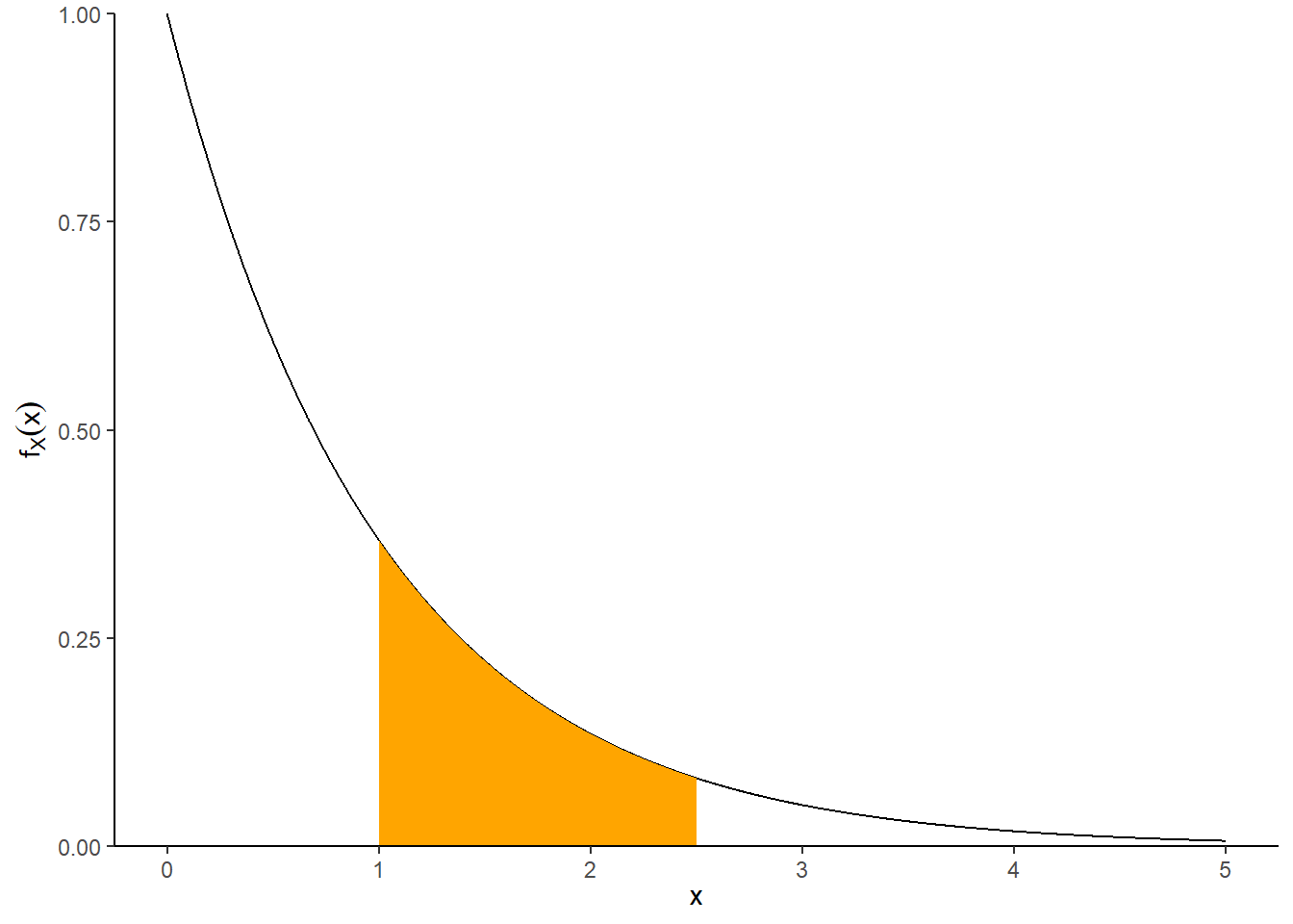
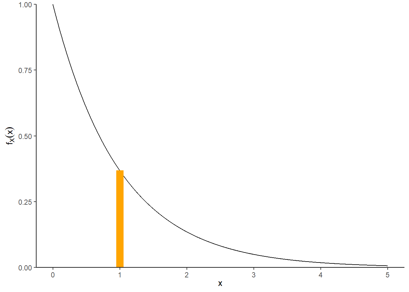
Figure 4.5: Illustration of $\textrm{P}(1<X<2.5)$ (left) and $\textrm{P}(0.995<X<1.005)$ (right) for $X$ with an Exponential(1) distribution, correspoding to the spinner in Figure 3.11. The plot on the left displays the true area under the curve. The plot on the right illustrates how the probability that $X$ is “close to” $x$ can be approximated by the area of a rectance with height equal to the density at $x$, $f_X(x)$.

A density is an idealized mathematical model. In practical applications, there is some acceptable degree of precision, and events like “$X$, rounded to 4 decimal places, equals 0.5” correspond to intervals that do have positive probability. For continuous random variables, it doesn’t really make sense to talk about the probability that the random value equals a particular value. However, we can consider the probability that a random variable is close to a particular value.

To emphasize: The density $f_X(x)$ at value $x$ is not a probability. Rather, the density $f_X(x)$ at value $x$ is related to the probability that the RV $X$ takes a value “close to $x$” in the following sense⁶⁷. $$\textrm{P}\left(x-\frac{\epsilon}{2} \le X \le x+\frac{\epsilon}{2}\right) \approx f_X(x)\epsilon, \qquad \text{for small $\epsilon$}$$ The quantity $\epsilon$ is a small number that represents the desired degree of precision. For example, rounding to two decimal places corresponds to $\epsilon=0.01$.

Technically, any particular $x$ occurs with probability 0, so it doesn’t really make sense to say that some values are more likely than others. However, a RV $X$ is more likely to take values close to those values that have greater density. As we said previously, what’s important about a pdf is relative heights. For example, if $f_X(\tilde{x})= 2f_X(x)$ then $X$ is roughly “twice as likely to be near $\tilde{x}$ than to be near $x$” in the above sense. $$\frac{f_X(\tilde{x})}{f_X(x)} = \frac{f_X(\tilde{x})\epsilon}{f_X(x)\epsilon} \approx \frac{\textrm{P}\left(\tilde{x}-\frac{\epsilon}{2} \le X \le \tilde{x}+\frac{\epsilon}{2}\right)}{\textrm{P}\left(x-\frac{\epsilon}{2} \le X \le x+\frac{\epsilon}{2}\right)}$$

4.3.1 Joint probability density fuctions

Recall that the joint distribution of random variables $X$ and $Y$ (defined on the same probability space) is a probability distribution on $(x, y)$ pairs. The joint distribution of two continuous random variables can be specified by a joint pdf, a surface specifying the density of $(x, y)$ pairs. The probability that the $(X,Y)$ pair of random variables lies is some region is the volume under the pdf surface over the region.

Example 4.15 Recall the example in Section 3.8.3. Let $\textrm{P}$ be the probability space corresponding to two spins of the Uniform(1, 4) spinner, and let $X$ be the sum of the two spins, and $Y$ the larger spin (or the common value if a tie). Review the results of the simulation in Section 3.8.3 before proceeding.

1. Find the joint pdf of $(X, Y)$. Hint: see Figure 3.14.
2. Use geometry to find $\textrm{P}(X <4, Y > 2.5)$.
3. Suggest an expression for the marginal pdf of $Y$. Hint: see Figure 3.16.
4. Use calculus to derive $f_Y(2.5)$, the marginal pdf of $Y$ evaluated at $y=2.5$.
5. Use calculus to derive $f_Y$, the marginal pdf of $Y$.
6. Find $\textrm{P}(Y > 2.5)$.
7. Suggest an expression for the marginal pdf of $X$. Hint: see Figure 3.15.
8. Use calculus to derive $f_X(4)$, the marginal pdf of $X$ evaluated at $x=4$.
9. Use calculus to derive $f_X(6.5)$, the marginal pdf of $X$ evaluated at $x=6.5$.
10. Use calculus to derive $f_X$, the marginal pdf of $X$. Hint: consider $x<5$ and $x>5$ separately.
11. Find $\textrm{P}(X < 4)$.
12. Find $\textrm{P}(X < 6.5)$.

Solution. to Example 4.15

Show/hide solution

1. Recall the discussion in Section 3.8.3. While marginally $X$ takes values in (2, 8) and marginally $Y$ takes values in (1, 4), not every pair in $(2,8)\times(1,4)$ is possible. Rather, the possible values of $(X, Y)$ lie in $\{(x, y): 2<x<8, 1<y<4, x/2<y<x-1\}$. The joint density of $(X, Y)$ is constant over the range of possible values. The region $\{(x, y): 2<x<8, 1<y<4, x/2<y<x-1\}$ is a triangle with area 4.5. The joint pdf is a surface of constant height floating above this triangle. The volume under the density surface is the volume of this triangular “wedge”. If the constant height is $1/4.5 = 2/9\approx 0.222$, then the volume under the surface will be 1. Therefore, the joint pdf of $(X, Y)$ is $$f_{X, Y}(x, y) = \begin{cases} 2/9, & 2<x<8,\; 1<y<4,\; x/2<y<x-1,\\ 0, & \text{otherwise} \end{cases}$$
2. $\textrm{P}(X <4, Y > 2.5) = 1/36$. The probability is the volume under the pdf over the region of interest. The base of the triangular wedge is $\{(x, y): 3.5<x<4, 2.5<y<3, x/2<y\}$, a region which has area $(1/2)(4-3.5)(3-2.5) = 1/8$. Therefore, the volume of the triangular wedge that has constant height 2/9 is $(2/9)(1/8) = 1/36$
3. The density starts at 0 at $y=1$ and then increases linearly until $y=4$. So we might guess $$f_Y(y) = \begin{cases} c(y - 1), & 1<y<4,\\ 0, & \text{otherwise.} \end{cases}$$ Then find $c$ to make the total area under the pdf equal 1. The area under the pdf is the area of a triangle with base 4-1 and height $c(4-1)$ so setting $1=(1/2)(4-1)(c(4-1))$ yields $c=2/9$.
4. We find the marginal pdf of $Y$ evaluated at $y=2.5$ by “stacking” the density at each pair $(x, 2.5)$ over the possible $x$ values. For discrete variables, the stacking is achieved by summing the joint pmf over the possible $x$ values. For continuous random variables we integrate the joint pdf over the possible $x$ values corresponding to $y=2.5$. If $y=2.5$ then $3.5 < x< 5$. “Integrate out the $x$’s” by computing a $dx$ integral: $$f_Y(0.25) = \int_{3.5}^5 (2/9)\, dx = (2/9)x \Bigg|_{x=3.5}^{x=5} = 1/3$$ This agrees with the result of plugging in $y=2.5$ in the expression in the previous part (with $c=2/9$).
5. To find the marginal pdf of $Y$ we repeat the calculation from the previous part for each possible value of $y$. Fix a $1<y<4$, and replace 2.5 in the previous part with a generic $y$. The possible values of $x$ corresponding to a given $y$ are $y + 1 < x < 2y$. “Integrate out the $x$’s” by computing a $dx$ integral. Within the $dx$ integral, $y$ is treated like a constant. $$f_Y(y) = \int_{y+1}^{2y} (2/9)\, dx = (2/9)x \Bigg|_{x=y+1}^{x=2y} = (2/9)(y-1), \qquad 1<y<4$$
6. If we have already derived the marginal pdf of $Y$, we can treat this just like a one variable problem. Integrate the pdf of $Y$ over $(2.5, 4)$ $$\textrm{P}(Y > 2.5) = \int_{2.5}^4 (2/9)(y-1)\, dy = (1/9)(y-1)^2\Bigg|_{y=2.5}^{y=4} = 0.25$$
7. We see that the density is 0 at $x=2$ and $x=8$ and has a triangular shape with a peak at $x=5$. If $c$ is the density at $x=5$, then $1 = (1/2)(8-2)c$ implies $c=1/3$. We might guess $$f_X(x) = \begin{cases} (1/9)(x-2), & 2 < x< 5,\\ (1/9)(8-x), & 5<x<8,\\ 0, & \text{otherwise.} \end{cases}$$ We could also write this as $f_X(x) = 1/3 - (1/9)|x - 5|, 2<x<8$.
8. We find the marginal pdf of $X$ evaluated at $x=4$ by “stacking” the density at each pair $(4, y)$ over the possible $y$ values. For discrete variables, the stacking is achieved by summing the joint pmf over the possible $y$ values. For continuous random variables we integrate the joint pdf over the possible $y$ values corresponding to $x=4$. If $x=4$ then $2 < y< 3$. “Integrate out the $y$’s” by computing a $dy$ integral: $$f_X(4) = \int_{2}^3 (2/9)\, dy = (2/9)y \Bigg|_{y=2}^{y=3} = 2/9 \approx 0.222$$ This agrees with the result of plugging in $x=4$ in the expression in the previous part.
9. This is similar to the previous part, but for $x=6.5$, we hit the upper bound of 4 on $y$ values; that is, the range isn’t just from $x/2$ to $x-1$, but rather $x/2$ to 4. If $x=6.5$ then $3.25 < y< 4$. “Integrate out the $y$’s” by computing a $dy$ integral: $$f_X(6.5) = \int_{3.25}^4 (2/9)\, dy = (2/9)y \Bigg|_{y=3.25}^{y=4} = 1/6 \approx 0.167$$ This agrees with the result of plugging in $x=6.5$ in the expression in two parts ago.
10. For $2<x<5$ the bounds on possible $y$ values are $x/2$ to $x-1$ $$f_X(x) = \int_{x/2}^{x-1} (2/9)\, dy = (2/9)y \Bigg|_{y=x/2}^{y=x-1} = (1/9)(x - 2), \qquad 2<x<5.$$ For $5<x<8$ the bounds on possible $y$ values are $x/2$ to $4$ $$f_X(x) = \int_{x/2}^{4} (2/9)\, dy = (2/9)y \Bigg|_{y=x/2}^{y=4} = (1/9)(8 - x), \qquad 5<x<8.$$ So the calculus matches what we did a few parts ago.
11. If we have already derived the marginal pdf of $X$, we can treat this just like a one variable problem. Integrate the pdf of $X$ over $(2, 4)$ $$\textrm{P}(X < 4) = \int_{2}^4 (1/9)(x-2)\, dx = (1/18)(x-2)^2\Bigg|_{x=2}^{x=4} = 2/9 \approx 0.222$$
12. If we have already derived the marginal pdf of $X$, we can treat this just like a one variable problem. It’s easiest to use the complement rule and integrate the pdf of $X$ over $(6.5, 8)$ $$\textrm{P}(X < 6.5) = 1 - \textrm{P}(X > 6.5) = 1 - \int_{6.5}^8 (1/9)(8-x)\, dx =1 - (-1/18)(8-x)^2\Bigg|_{x=6.5}^{x=8} = 1 - 1/8 = 7/8 = 0.875$$

Definition 4.4 The joint probability density function (pdf) of two continuous random variables $(X,Y)$ defined on a probability space with probability measure $\textrm{P}$ is the function $f_{X,Y}:\mathbb{R}^2\mapsto[0,\infty)$ which satisfies, for any $S\subseteq \mathbb{R}^2$, $$\textrm{P}[(X,Y)\in S] = \iint\limits_{A} f_{X,Y}(x,y)\, dx dy$$

A joint pdf is a surface with height $f_{X,Y}(x,y)$ at $(x, y)$. The probability that the $(X,Y)$ pair of random variables lies in the region $A$ is the volume under the pdf surface over the region $A$

A joint pdf is a probability distribution on $(x, y)$ pairs. The height of the density surface at a particular $(x,y)$ pair is related to the probability that $(X, Y)$ takes a value “close to⁶⁸” $(x, y)$ $$\textrm{P}(x-\epsilon/2<X < x+\epsilon/2,\; y-\epsilon/2<Y < y+\epsilon/2) = \epsilon^2 f_{X, Y}(x, y) \qquad \text{for small $\epsilon$}$$

A valid joint pdf must satisfy $$\begin{align*} f_{X,Y}(x,y) & \ge 0\\ \int_{-\infty}^\infty\int_{-\infty}^\infty f_{X,Y}(x,y)\, dx dy & = 1 \end{align*}$$ Given a specific pdf, the generic bounds $(-\infty, \infty)\times(-\infty, \infty)$ in the above integral should be replaced by the range of possible pairs of values, that is, those $(x, y)$ pairs for which $f_{X, Y}(x, y)>0$.

The marginal pdfs can be obtained from the joint pdf by the law of total probability. In the discrete case, to find the marginal probability that $X$ is equal to $x$, sum the joint pmf $p_{X, Y}(x, y)$ over all possible $y$ values. The continuous analog is to integrate the joint pdf $f_{X,Y}(x,y)$ over all possible $y$ values to find the marginal density of $X$ at $x$. This can be thought of as “stacking” or “collapsing” the joint pdf.

$$\begin{align*} f_X(x) & = \int_{-\infty}^\infty f_{X,Y}(x,y) dy & & \text{a function of $x$ only} \\ f_Y(y) & = \int_{-\infty}^\infty f_{X,Y}(x,y) dx & & \text{a function of $y$ only} \end{align*}$$

The marginal distribution of $X$ is a distribution on $x$ values only. For example, the pdf of $X$ is a function of $x$ only (and not $y$). (Similarly the pdf of $Y$ is a function of $y$ only and not $x$.)

In general the marginal distributions do not determine the joint distribution, unless the RVs are independent. In terms of a table: you can get the totals from the interior cells, but in general you can’t get the interior cells from the totals.

---

65. The same is not true for discrete random variables. For example, if $X$ is the number of heads in three flips of a fair coin then $\textrm{P}(X<1)= \textrm{P}(X=0)=1/8$ but $\textrm{P}(X \le 1)=\textrm{P}(X=0)+\textrm{P}(X=1) = 4/8$.↩︎

66. Reporting so many decimal places is unnecessary, and provides a false sense of precision. All of these idealized mathematical models are at best approximately true in practice. However, we provide the extra decimal places here to compare the approximation with the “exact” calculation.↩︎

67. This is true because an integral is really just a sum of the areas of many rectangles with narrow bases. Over a small interval of values surrounding $x$, the density shouldn’t change that much, so we can estimate the area under the curve by the area of the rectangle with height $f_X(x)$ and base each equal to the length of the small interval of interest.↩︎

68. You can have different precisions for $X$ and $Y$, e.g., $\epsilon_x, \epsilon_y$, but using one $\epsilon$ makes the notation a little simpler.↩︎