11 Getting data
Where does data come from? In the vast majority of cases, the data we analyze was not generated by ourselves. Instead, we are provided with or find data that is of interest to us. As such data may stem from a variety of sources, it is usually not pre-processed or saved by R. Thus, a non-trivial question that needs to be answered is: How can we get this data into R?
In R, we generally get data — typically in the form of vectors or tables — by either importing it from some file or by creating it from scratch. In both cases, we usually want to end up with a rectangular data structure known as a tibble, which is a simplified version of an R data frame.
The two key topics of this chapter are:
Reading and writing data files with the readr package (Wickham, Hester, et al., 2023)
Creating tibbles with the tibble package (Müller & Wickham, 2023)
As both these packages belong to the tidyverse (Wickham et al., 2019), they create a rectangular data structure known as a tibble. While these packages are more consistent and convenient than the corresponding base R functions, the utils package also contains generic functions for reading and writing files, and we could get by just fine by only using data frames, rather than tibbles.
An important precondition for working productively with R (or any other programming language) is that we have some basic understanding of file systems and storage locations. Thus, this chapter needs to briefly explain the notion of (absolute or relative) paths and how to organize R projects.
Preparation
Recommended readings for this chapter include
of the ds4psy book (Neth, 2023a).
For a more comprehensive overview, see
of the r4ds book (Wickham & Grolemund, 2017).
Preflections
Before reading, please take some time to reflect upon the following questions:

If we were interested in answering some interesting question, what data would we require?
Where do we get data from?
If someone had all the data we need, how would we obtain, load or enter it into R?
How can we load a data file from another directory or a different machine?
How would we store or share our data?
In this chapter, we will learn how to orient ourselves on our computer, and how to create, read, and write tabular data structures in R.
11.1 Introduction
Data is rarely entered directly into R. When we analyze data, getting data into R can either imply
importing data from some file or server (see Section 11.3), or
creating data from scratch (see Section 11.4).
In both cases, we aim to end up with rectangular data structure known as a “tibble”, which is a simplified type of data frame, used in the tidyverse (Wickham et al., 2019). But tibbles are not just an end result of getting and analyzing data — we may also want to share them with others. This requires saving (or “writing”) our data to files into some folder in a form that allows us or others to re-load them (into R or other programs).
A typical R workflow includes not only reading and writing files, but also that we are oriented in our current computing environment. This implies that we can navigate between folders, can describe and link to files, and know how to organize an R project (see Section 11.2).
Key concepts
Key concepts of Section 11.2 on getting oriented and organized include:
- files and folders
- R’s working directory
- paths (absolute vs. relative)
- R projects
Key concepts of Section 11.3 on importing data include:
- parsing (vectors or files)
- importing/reading vs. exporting/writing files
Key concepts of Section 11.4 on creating tibbles include:
- rectangular data structures (with rows/cases and columns/variables)
- data frames vs. tibbles
- data types: logical, character, or numeric variables vs. factors
Resources
Resources for Section 11.3 on importing data include:
The base R package utils and the tidyverse package readr (Wickham, Hester, et al., 2023)
Chapter 6: Importing data of the ds4psy book (Neth, 2023a).
Chapter 11: Data import of the r4ds book (Wickham & Grolemund, 2017).
Resources for Section 11.4 on creating tibbles include:
The R package tibble (Müller & Wickham, 2023)
Chapter 5: Tibbles of the ds4psy book (Neth, 2023a).
Chapter 10: Tibbles of the r4ds book (Wickham & Grolemund, 2017).
Before we can begin to import data into R, we need to get oriented on our computers.
11.2 Getting oriented and organized
Modern computer systems usually provide some sort of graphical user interface, that visualizes the contents of our hard drives as files that are stored in directories (or folders). Given fancy interactive devices (like a mouse or a track pad), the task of navigating between folders and moving files becomes a perceptual-motor task that involves clicks and gestures. Although this may be more convenient than typing into a terminal, some knowledge of location descriptions (or “paths”) is helpful when working with R (or any other programming language).
Our R system operates within an infrastructure that consists of many files and folders, but also other programs and computers. When adopting the perspective of our R system, we can always ask:
- Where am I?
- Where is the data?
The answer to the first question is known as R’s current working directory.
As we can start R from various locations (e.g., locally or on a remote server), the working directory is not necessarily the same directory as the location of an R file that we are editing or evaluating.
A well-organized project typically contains various (sub-)directories for storing different types of data.
For instance, larger projects contain dedicated sub-directories for data, images, or R code files.
To determine the current working directory, we can use the getwd() function of base R.
For the i2ds book, the working directory is:
getwd()
#> [1] "/Users/hneth/Desktop/stuff/Dropbox/GitHub/i2ds_book"
Note that evaluating the getwd() function returns a directory path, which is the description of a location on a computer (as a character string). This path depends both on our operating system (e.g., its hierarchy of directories) and on the specific organization of our local file system.
If we wanted to change R’s working directory, we could use the setwd() function and provide an alternative location in its dir argument. For instance, the following code would first save R’s current working directory (as wd) and then change it to another directory, before changing it back to the original directory:
# 0. store original working directory:
wd <- getwd()

# 1. Change to a different working directory:
setwd(dir = "/Users/hneth/Desktop/stuff/")
getwd()  # verify new working directory
#> [1] "/Users/hneth/Desktop/stuff"

# 2. Re-set original working directory:
setwd(wd)
Given such functions to find out and change our working directory, we can ask:
- Why would we want to know or change our working directory?
The fact that we often work with multiple projects and not all files are stored in the same directory make it necessary to know or set one’s current working directory, as well as point to the locations of files in other directories. When working with projects in the RStudio IDE, R sets a session’s original working directory to the project folder.
11.2.1 Local vs. remote files
The reason to know and possibly change our working directory is that we frequently need to access (e.g., read or write) files that are located elsewhere (i.e., in other directories). The notion of “elsewhere” is deliberately vague: If we only consider files within our working directory as “local”, all other files are “remote”. Thus, a remote file A can be located in a sub-directory of our working directory and a remote file B on an online server at the other end of the world. From R’s perspective, both files are remote by not being located in the working directory.
The list.files() function shows us the local files of a directory.
For instance, to see the files and directories of our working directory, we could evaluate:
list.files() # list local files and directoriesWhen aiming to access a remote file, we could change our working directory to this other location, so that the file becomes local. However, the more common way of dealing with such situations is to retain our current working directory and describe the location of the remote file by its path.
11.2.2 Absolute vs. relative paths
The second question from above (“Where is the data?”) can be answered in two ways, but both involve specifying a path to the data. File paths are descriptions of locations on a computer, typically expressed as character strings. Whenever aiming to read or write files that are not stored in our current working directory, we need to specify their path. Similarly, linking between files or to media contents (e.g., an image) requires providing their file paths.
We can distinguish between two types of file paths:
absolute paths are a top-down description of locations (or the “address” of a file or directory) on a computer. Unfortunately, the way in which file paths are expressed can vary between computer operating systems (but we can always evaluate
getwd()in R to see how our own computer expresses absolute paths). Absolute paths always include the root directory of a particular machine. On UNIX-like systems, the root directory is denoted by/(i.e., a forward slash). When accessing a file from an online server, its absolute path may include elements of URL addresses (likehttpsorwww).relative paths are descriptions of locations (or the “address” of a file or directory) relative to the current working directory. For instance, if my current working directory was
/Users/hneth/project_1, then"/data/my_data.tab"(as a character string) provides a relative path to a filemy_data.tabthat is located in adatasub-directory of theproject_1directory. Thus, the absolute path of this file is/Users/hneth/project_1/data/my_data.tab.
When specifying file paths, some abbreviations are helpful. The most common ones are:
.(i.e., the dot symbol) denotes the current location (i.e., working directory)..(i.e., two dot symbols) denote the current parent directory (i.e., “one level up in the hierarchy”)~(i.e., the squiggly tilde symbol) denotes a user’s home directory
As . and .. are always interpreted relative to the current location, they are used when specifying relative (or local) paths. By contrast, ~ is an abbreviation for an absolute (or global) path.
Importantly, absolute and relative paths can point to the same locations — they really are just two different ways of pointing to an address (typically directories or files on our computer). But as local paths are always interpreted relative to the current working directory, the same local path points to different locations when we begin in a different working directory.
Thinking of two different locations on a map may help: To find out how to get from our current location \(A\) to another location \(B\), we can either look up the absolute/global address of \(B\) (i.e., using street names, numbers, or the map’s coordinate system) or provide directions in a relative/local fashion by adopting \(A\)’s perspective (i.e., “keep going, turn right on the 2nd street, then straight ahead, before turning left at…”). Whereas the absolute address of \(B\) is independent of our current location \(A\), providing relative directions (e.g., “turn right”) assumes knowledge of our current location \(A\). Thus, although the absolute and relative descriptions differ, they can both get us from \(A\) to \(B\).
If both types of file paths can describe the same location, why does their difference matter for us? Importantly, global paths always contain the top-level directories of a particular computer, whereas local paths ignore top-level details. As long as all files that belong together are transferred together with their directory structure, local paths are preferable (an work in the same way as local directions do, provided that we know our initial location and direction). By contrast, global file paths differ between different computers and should be avoided in our code (or must be clearly marked as being user-specific, if they are being used).
11.2.3 Organizing R projects
As R projects typically consist of multiple files and folders, we need to care about file paths when we ever want to share code or transfer projects to a different machine. The following strategy is based on design principles of websites, which face and solve the same problem:
Anchor every project in a home directory and identify this directory by its absolute path.
Store all files belonging to the project in sub-directories of the home directory, and identify these files by using their relative paths (e.g., express all links to data or image files relative to the home directory).
When accessing to external files (i.e., files not stored within the home directory), refer to these files by their absolute paths (and identify them prominently, e.g., at the top of your main project file).
Following these guidelines makes an R project as self-contained and transferable as possible.
Similar strategies are adopted for designing R packages
(for details, see the Section on Package subdirectories in the manual on Writing R extensions) or when we use the
RStudio IDE for defining a “project”.
The key advantage of these principles is that we can transfer an entire project from one location to another (on the same or a different machine). Once we re-set the project’s home directory (e.g., by calling getwd() or by using the here() function of the here package), everything else continues to work (provided that we transferred the entire content of the home directory and only used local paths to identify files in its sub-folders).
If our project needs to access files from external projects or locations that cannot be easily stored within our project (e.g., data files that are too large to copy or images that are being hosted on external servers), it is useful to store their paths as R objects that provide their absolute paths. For instance, the source code of this book defines R objects for the current URLs of the ds4psy and i2ds textbooks (as character strings):
url_ds4psy_book <- "https://bookdown.org/hneth/ds4psy/"
url_i2ds_book   <- "https://bookdown.org/hneth/i2ds/"
The advantage of specifying external URLs as R objects within our project is that we only need to change the object definition once, if the online address of our project changes (which is quite common for web addresses).
As both these directories contain sub-directories for data and images, we can link to their files by specifying either their local or their global paths.
When working on the i2ds project, it is preferable to use a relative file path to link to its cover image:
# (a) include an image (as a relative/local link):
my_image <- "./images/cover.png"  # use local path
knitr::include_graphics(path = my_image)
Figure 11.1: A local image identified by its relative path.
Incidentally, the expression knitr::include_graphics() is a way to call the include_graphics() function of the knitr package. Thus, expressions like pkg::fun() are yet another way to denote paths in R (in this case, the call is interpreted relative to our current library of R packages).
However, when aiming to show an image from a different project (e.g., from the ds4psy textbook), it is better to specify and use its global path (even if we had access to the file on our local computer). Assuming that we know its location, we could do this by specifying its absolute path as an R object:
# (b) include an image (via absolute/global link):
my_image <- paste0(url_ds4psy_book, "/images/cover.png")   # use global path
my_image <- paste0(url_ds4psy_book, "/", "images", "/", "cover.png")
knitr::include_graphics(path = my_image)
Figure 11.2: An external image identified by its absolute path.
As file paths are of data type “character” (i.e., strings of text), we can use text manipulation functions like paste0() to compose and modify them.
As always, there are tools that help us organize our projects:
Defining a “project” within the RStudio IDE automatically sets R’s working directory to the project directory. As long as all files needed in the project are identified as relative paths, such projects can easily be transferred between locations. See Chapter 8 Workflow: projects of the r4ds textbook (Wickham & Grolemund, 2017) for instructions.
The here package (Müller, 2017) simplifies working with file paths, but also requires a basic understanding of them.
Overall, many of these concepts and steps may seem trivial to experienced computer users. Ideally, knowing and navigating the organizational structure of one’s machine and R projects should become as habitual as other daily routines. To sum up, let’s briefly recapitulate what this section has taught us:
Summary: Getting oriented and organized
Programs and data on computers are typically structured within a hierarchy of files and folders. As R code usually involves many different files, they are usually structured into packages or projects, with dedicated directory and file structures.
R runs in its working directory, which can be identified by
getwd()and changed bysetwd().The storage locations of files in folders are identified by paths (as character strings), which can be absolute (global) or relative (local).
-
To be as self-contained and transferable as possible, R projects should be organized as follows:
- An R project’s working directory should be identified by its absolute path.
- All files within a project should be identified by their relative paths.
- Any external files should be clearly identified and expressed as absolute paths (e.g., URLs).
11.2.4 Practice
Solution
# (a) Getting and setting working directories:
getwd()        # print (absolute) file path of current working directory
wd <- getwd()  # store current file path
setwd("/")     # set working directory to root directory
setwd(wd)      # reset working directory (to wd from above)

# (b) Navigating relative file paths:
setwd(".")       # no change (as "." marks current location)
setwd("./data")  # move 1 level down into "data" (if "data" exists)
setwd("..")      # move 1 level up (from current directory)
setwd("./..")    # move another level up (from current directory)

# (c) Assuming 2 sub-directories ("./code" and "./data"):
setwd("code")     # move down into directory "code"
setwd("../data")  # move into parallel directory "data"
setwd("../code")  # move into parallel directory "code"
setwd("..")       # move 1 level up
Organizational concepts
Answer the following questions in your own words:
- Which tasks are being solved by file paths?
- What is the difference between absolute and relative paths?
- Why is it smart to rely on relative paths within an R project?
- When does it still make sense to use absolute paths in an R project?
11.3 Importing data
Importing data is one of the most important, but also most mundane steps in analyzing data. Unfortunately, anything that goes wrong at this step is likely to affect everything else that follows.
As we typically deal with tabular (or rectangular) data, the utils package of R contains a range of read.table() functions that read files into data frames from various formats. The most commonly used of these are:
read.csv()andread.csv2for importing comma-separated value (csv) filesread.delim()andread.delim2()for importing other delimited files (e.g., using the TAB character to separate the values of different variables)read.fwf()for reading fixed width format (fwf) files
The readr package of the tidyverse provides similar and additional functions for reading (or “parsing”) vectors and importing data files into a simplified type of data frame (known as a tibble).
Both the utils and the readr packages also provide a range of write() functions that allow exporting (and storing) data files in various formats.
Importing and exporting files also assume some knowledge about how to denote paths to files or computer locations (on a local file systems or remote servers).
As these topics are covered in Chapter 6: Importing data, the rest of this section only contains some excerpts and examples. Additional details are available in the following sections of the ds4psy book (Neth, 2023a):
Section 6.1.2 Orientation and navigation describes how to denote paths.
Section 6.2 Essential readr commands introduces key readr functions.
11.3.1 Reading and writing files
The main way to get data into R is by importing (or “reading”) data files. Doing this requires not only the existence of the file, but also knowing its storage location. Storage locations can be local (on our own computer) or remote (on some online server), with various intermediate cases (e.g., on another drive or computer on the same network).
In R, all functions that read or write files use a flexible file argument that typically describes a path to a file (as a character string), but can also specify a connection (to a server), or even literal data (as a single string or a raw vector).
Key readr functions include:
read_csv()vs.read_csv2()for reading comma-separated data filesread_delim()for reading data files not delimited by commaswrite_csv()vs.write_csv2()for writing comma-separated data fileswrite_delim()for writing data files not delimited by commas
These commands and corresponding examples are illustrated in Section 6.2.2 Parsing files of the ds4psy book (Neth, 2023a).
Dealing with problems:
- For parsing vectors, see Section 11.3 Parsing a vector of the r4ds book (Wickham & Grolemund, 2017) or Section 6.2.1 Parsing vectors of the ds4psy book (Neth, 2023a).
11.4 Creating tibbles
In Chapter 3 on Data structures, we combined vectors of the same length into a special type of rectangular data structure that was called a data frame. Internally, such tables are represented as a list of vectors and their elements (i.e., cells, columns, or rows) and can be accessed by logical or numeric subsetting. Whenever we load (i.e., parse or read) rectangular data into R, a desirable data structure of the resulting object is a data frame or a tibble.
Tibbles are simple data tables and the primary way of representing data (in rows of cases and columns of variables) in the tidyverse (Wickham, 2023). Internally, tibbles are a special, simplified form of a data frame.
How can we create tibbles from other rectangular data structures (e.g., vectors or data frames)? And what can we do not yet have another rectangular table, but want to create a tibble from scratch?
Key tibble functions include:
as_tibble()converts (or coerces) an existing rectangle of data (e.g., a data frame or matrix) into a tibble.tibble()converts several vectors into (the columns of) a tibble.tribble()converts a table (entered row-by-row) into a tibble.
Thus, the three functions differ by the types of inputs they expect, but have in common that they create a tibble as their output.
While some R veterans may prefer data frames, tibbles are becoming increasingly popular.
But if we ever need to transform a tibble tb into a data frame, we can always use as.data.frame(tb).
These commands and corresponding examples are illustrated in Section 5.2 Essential tibble commands of the ds4psy book (Neth, 2023a).
11.5 Conclusion
11.5.1 Summary
An R process always runs in some working directory. Getting data into R (or any other computing system) assumes a basic understanding of files, folders, and paths (i.e., descriptions of their locations, typically in the form of character strings).
The R packages readr and the tibble provide functions for creating data structures known as “tibbles” in R. For our purposes, tibbles are a simpler and well-behaved data frames. More specifically,
readr provides functions for reading data (stored as vectors or rectangular tables) into tibbles;
tibble provides functions for getting tibbles from other data structures (data frames, vectors, or row-wise tables).
11.5.2 Resources

Figure 11.3 shows the RStudio cheatsheet on importing and exporting data:
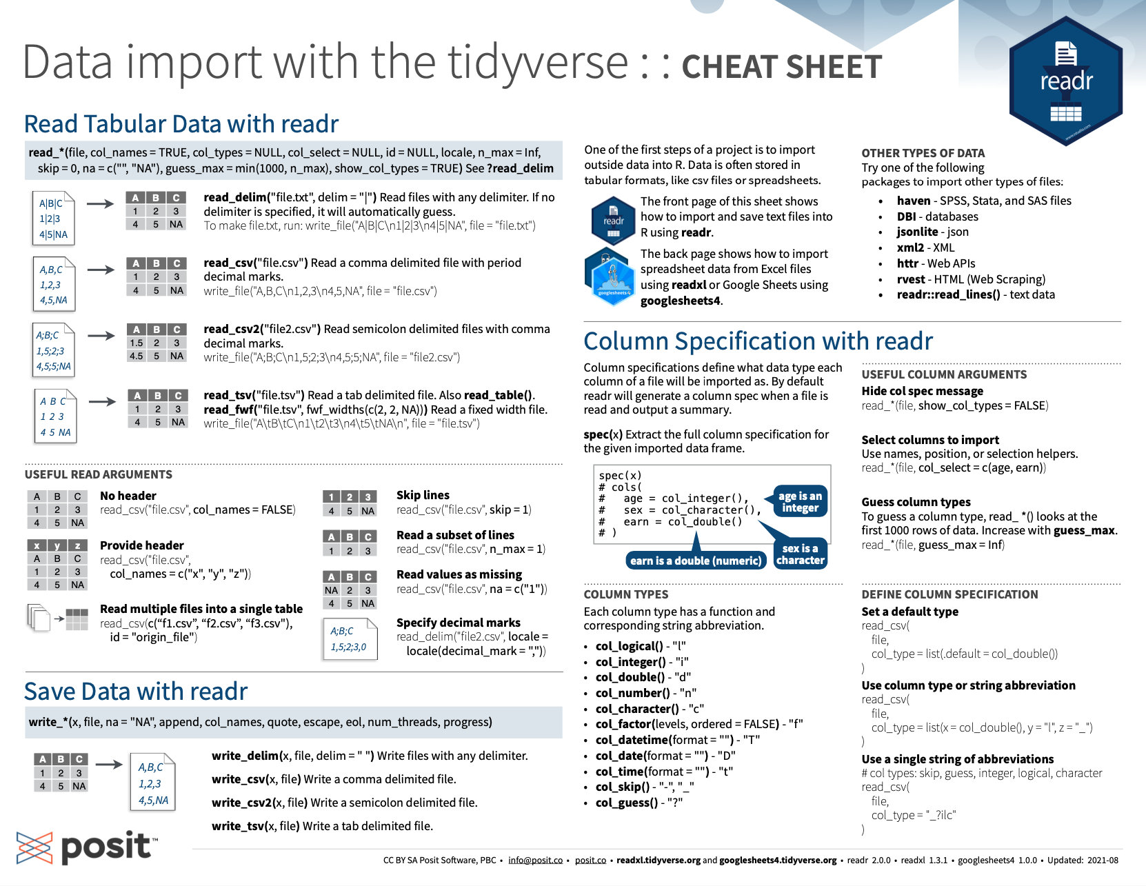
Figure 11.3: The RStudio cheatsheet on importing and exporting data with the readr package.
Figure 11.4 shows the back of the cheatsheet shown in Figure 11.3:
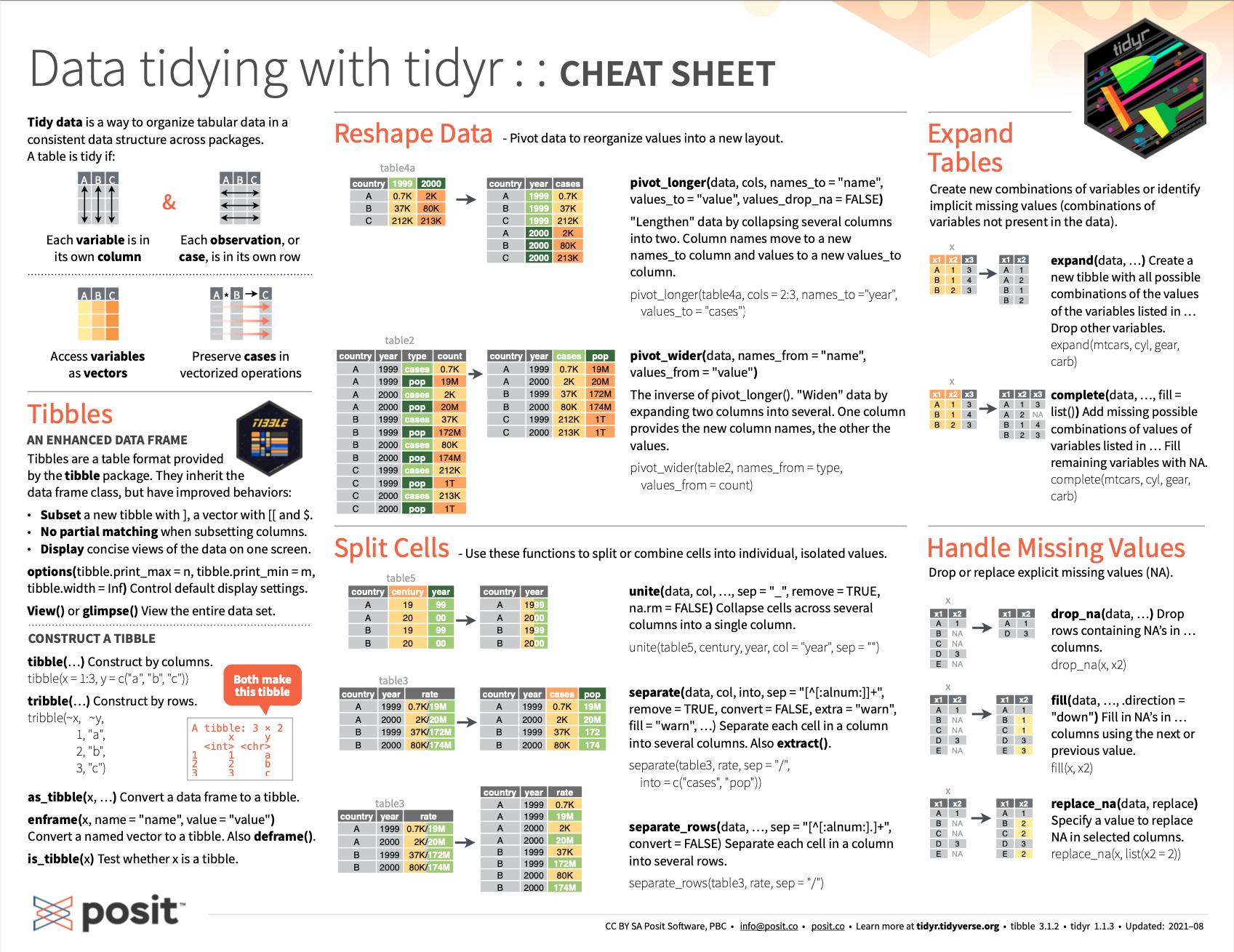
Figure 11.4: Essential tibble commands on the RStudio cheatsheet on the tidyr package.
The fact that both tibble and tidyr are covered by the same RStudio cheatsheet on Data tidying show the close correspondence between both topics.
11.5.3 Preview
The RStudio cheatsheet on Data Import also summarizes commands of a third package tidyr. This package starts with tibbles, but transforms them into different formats. A key concept in this context is the notion of tidy data.
In Chapter 12 on Transforming data, we will introduce the tidyr package and the dplyr package for data transformation. Just like readr and tibble, both packages are key components of the tidyverse (Wickham, 2023).
11.6 Exercises

The following exercises link to the corresponding exercises of Chapter 6: Importing data and Chapter 5: Tibbles. Please complete at least one exercise of each part (A, B, C).
11.6.2 Including images by absolute vs. relative links
Suppose you wanted to include an online image in your R Markdown file. To achieve this, you could either
- link to the online image by using its absolute path (to some web server), or
- copy the image into an
/imagesub-directory of your project and use the (absolute or relative) link to this location.
- copy the image into an
Discuss the advantages and disadvantages of both options.
Implement both options for an example image.
Part C: Creating tibbles
At least two exercises (out of three) from Chapter 5: Tibbles on the tibble package (Müller & Wickham, 2023):
11.6.6 Flower power
Parts 1, 3–5 (i.e., all except for Part 2) of Exercise 1 of Chapter 5: Tibbles
11.6.7 Rental accounting
Part 1 of Exercise 2 of Chapter 5: Tibbles
11.6.8 False positive psychology
Exercise 4 of Chapter 5: Tibbles
This concludes our exercises on importing data and creating tibbles.