Model 9: Demography and cultural gain / loss
Introduction
Demography refers to the study of populations: their size, structure, and movements in and out. We have already examined demography in previous models. This was most explicit in Model 7 where we looked at migration between two separate sub-populations. However, in all of the models so far, we have seen how small populations are more likely to lose traits purely by chance, while large populations have more stable dynamics that more closely match analytical models with infinite population sizes.
Here we will pursue this further by examining an influential model created by Henrich (2004) that links demography - specifically, population size, \(N\) - to cultural losses and cultural gains. Henrich (2004) did this in the context of an archaeological example. Around 12,000 years ago, Tasmania became cut off from the mainland of Australia due to rising sea levels. Upon first contact with European explorers, the Aboriginal Tasmanians had strikingly simple technology compared to the Aborigines of the mainland: they lacked bone tools, fishhooks, traps and nets, spearthrowers and boomerangs, all of which were used on the mainland. Henrich argued that this technological loss or stagnation was not because the Tasmanians were less smart or skilful than their mainland counterparts. Rather, it was because when they were cut off from the mainland their population size dropped dramatically. Tools such as fishhooks are hard to make, and subject to error. When there are few skilled fishhook-makers, fishhook technology is easily lost and unlikely to be reinvented. In large populations, however, there will be lots of skilled fishhook makers. Even if some forget or fail to pass on their fishhook-making skill, there will be others to carry on the tradition. This is an example of cumulative cultural evolution, where individuals acquire skills and knowledge from others that they could not invent on their own. While Henrich framed his model in the context of prehistoric Tasmania, we can generalise this principle to any case where hard-to-learn traits are dependent on population size.
Model 9
Henrich (2004) used a simple model to explore this scenario of cultural loss due to small population size. We assume \(N\) individuals who each possess a value of a continuously varying, culturally transmitted skill (e.g. fishhook making). This skill is denoted \(z_i\) for individual \(i\), where \(i\) ranges from 1 to \(N\). Note that, technically, \(N\) is the ‘effective’ population size. This is the number of individuals who would be able to possess the trait in question. It may be less than the actual (‘census’) population size if, for example, infants or some other class of individual do not or cannot make fishhooks.
In each new generation, every individual copies the \(z\) value of the most highly skilled individual from the previous generation, denoted \(z_h\). This is a form of biased transmission or cultural selection, similar to the payoff-based indirectly-biased transmission explored in Model 4. Here, demonstrators are preferentially selected based on their superior culturally-transmitted skill or knowledge.
If individuals perfectly copied the highest trait value from the previous generation, then the model would not be very interesting. It would also not be very realistic. Instead, we assume that this indirectly biased transmission is imperfect. It is imperfect in two ways. First, there is skill loss due to mistakes in the copying process. This always reduces the copier’s \(z\) value relative to the target \(z_h\). Second, there are experiments, guesses and inferences. These sometimes result in worse skill, but sometimes better skill than the target \(z_h\).
To formalise these two kinds of variation, Henrich (2004) assumed that naive learners’ skill \(z_i\) is drawn from a gumbel distribution. This is similar to the blending inheritance of Model 8 where we drew copied values from a normal distribution. A gumbel distribution is generated when extreme values are repeatedly picked. This is what we are doing when we pick the highest-skilled demonstrator to learn from in each generation, so it is more appropriate than a normal distribution.
Unfortunately R does not provide built-in functions to work with gumbel distributions. However, we can write our own, using the formula for the probability density of the distribution. The following functions, dgumbel and rgumbel, generate the probability density and random draws for a gumbel distribution. I won’t go into details on the formulae, but you can look them up if you want.
# probability density of the gumbel, for values x
# a is the mode, beta is the dispersion
# defaults to standard gumbel with a=0 and beta=1
dgumbel <- function(x, a = 0, beta = 1) {
  b <- (x - a)/beta
  (1/beta)*exp(-(b+exp(-b)))
}

# n random draws from a gumbel distribution with mode a and dispersion beta
# defaults to standard gumbel with a=0 and beta=1
rgumbel <- function(n, a = 0, beta = 1) {
  a + beta * (-log(-log(runif(n))))
}
Gumbel distributions take two parameters, a mode \(a\) and a dispersion \(\beta\). Here is an example gumbel distribution, with additional labels showing Henrich’s model parameters (recreating Fig 1 in Henrich 2004).
x <- seq(0,100,0.1)  # x-axis values
a <- 30  # mode
beta <- 15  # dispersion

# plot gumbel distribution for the parameters defined above
plot(x, dgumbel(x, a, beta),
     type = 'l',
     ylab = expression("Probability Imitator Acquires "*italic("z"[i])),
     xlab = expression("Imitator "*italic("z"[i])*" Value"),
     bty='l')

# add a vertical dotted line for the demonstrator with z_h
alpha <- 30
abline(v = a + alpha, lty=2)
text(a + alpha + 18, 0.02,
     labels = expression("Demonstrator "*italic("z"[h])*" value"))

# add beta label and arrows
text(a+2, 0.013,
     labels = expression(beta))
arrows(a+4, 0.013, a+19, 0.013, length=0.1)
arrows(a-1, 0.013, a-13, 0.013, length=0.1)

# add alpha label and arrows
text(a+alpha/2, 0.025,
     labels = expression(alpha))
arrows(a+2+alpha/2, 0.025, a+14+alpha/2, 0.025, length=0.1)
arrows(a-2+alpha/2, 0.025, a-14+alpha/2, 0.025, length=0.1)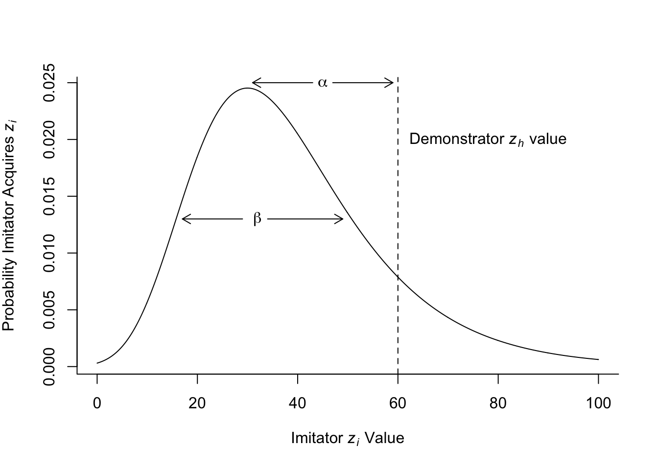
Notice how the gumbel distribution looks like an asymmetric normal distribution which is elongated at the upper end. This reflects the fact that we are sampling extreme high values. A demonstrator \(z_h\) value is shown on the plot with a dotted vertical line. This is the highest-skill value that the imitator is trying to copy. Their actual copied \(z_i\) value is drawn randomly from this gumbel distribution.
The \(\alpha\) parameter determines the first kind of deviation described above, the transmission error. This is the difference between the demonstrator \(z_h\) value and the mode of the gumbel distribution (which is \(a\) - try not to confuse the mode \(a\) with the transmission error parameter \(\alpha\). It’s not ideal notation, but I’ll stick with it because that’s what Henrich used. \(z_h\) is therefore \(a + \alpha\)). The larger is \(\alpha\), the further the mode will be below the \(z_h\) value, and the more likely the copied \(z_i\) value will be less than \(z_h\).
The \(\beta\) parameter is the dispersion of the gumbel distribution, controlling the width. This represents the second kind of deviation described above, the inferential guesses or experiments. The larger is \(\beta\), the more likely the copied \(z_i\) value will be different to the copied \(z_h\) value. Occasionally, the copied \(z_i\) value will be higher than the demonstrator \(z_h\) value. This occurs with probability equal to the area under the curve to the right of the dotted vertical line, in the extreme right-hand tail of the distribution. The larger is \(\beta\), the larger this area will be. So while \(\alpha\) always makes copied values worse than \(z_h\), \(\beta\) increases the chances that copied values will occasionally exceed \(z_h\).
Let’s simulate this model to confirm this, and find out when the mean skill in the population \(\bar z\) increases, representing cultural gain, and when it decreases, representing cultural loss.
The following function follows the structure of previous models. After repeating the rgumbel function definition from above (just to make sure that this function is defined, and make DemographyModel self-contained), first we set up an output dataframe. In this case the output dataframe needs to store the mean trait value \(\bar z\) in each generation from 1 to \(t_{max}\). Then we set up the agent dataframe: each of \(N\) agents’ initial trait value is randomly drawn from a gumbel distribution with mode 0 and dispersion \(\beta\). After storing the first generation mean trait value, we start cycling through generations. Each generation, we find the maximum skill value for the current generation \(z_h\), then draw \(N\) new agents from a gumbel distribution with mode \(z_h - \alpha\) and dispersion \(\beta\) as per the figure above and using rgumbel. Each generation we store the new mean trait value, before plotting them all at the end and outputting the data from the function. Note the use of expression() in the plot axis labels; this allows us to use italics, subscripts and bars in the plot text.
DemographyModel <- function(N, alpha, beta, t_max) {

  rgumbel <- function(n, a = 0, beta = 1) {
    a + beta * (-log(-log(runif(n))))
  }

  # create output dataframe to hold mean trait value for each generation
  output <- data.frame(z_bar = rep(NA, t_max))

  # create 1st generation, N random draws from a gumbel with mode a=0 and dispersion beta
  agent <- data.frame(trait = rgumbel(N, beta = beta))

  # store first generation trait mean
  output$z_bar[1] <- sum(agent$trait) / N

  for (t in 2:t_max) {

    # get highest skill from current generation
    z_h <- max(agent$trait)

    # draw new values
    agent$trait <- rgumbel(N, a = z_h - alpha, beta = beta)

    # store new mean trait value
    output$z_bar[t] <- sum(agent$trait) / N

  }

  plot(x = 1:nrow(output), y = output$z_bar,
       type = 'l',
       ylab = expression("mean trait value "*italic(bar("z"))),
       xlab = "generation",
       main = paste("N = ", N, ", alpha = ", alpha, ", beta = ", beta, sep = ""))

  output
}
Let’s run the demography model with the values of \(\alpha\) and \(\beta\) used in the first figure above, and \(N=100\):
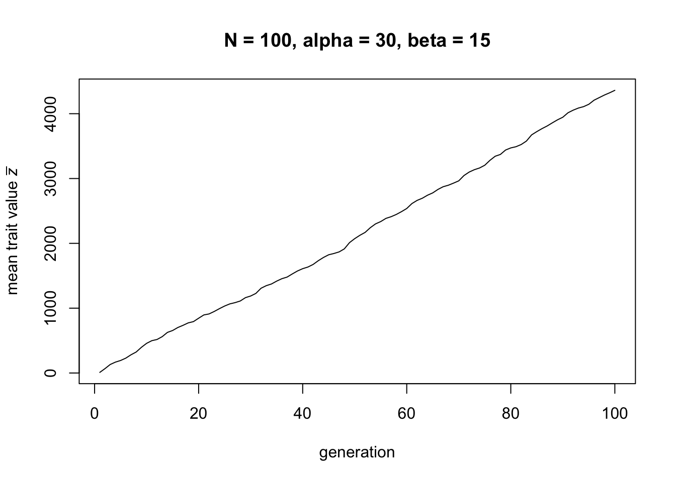
Here we can see that, for these parameter values, there is cultural gain: the mean trait value \(\bar z\) increases linearly over time.
Now let’s try the smallest population size possible, \(N = 1\):
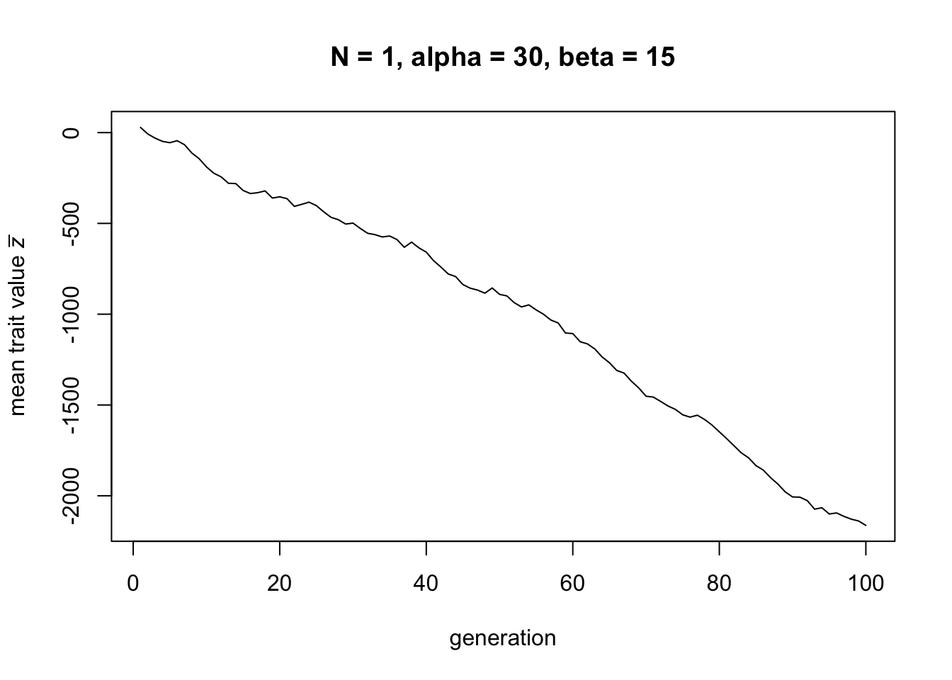
Now there is cultural loss: the mean trait value \(\bar z\) decreases linearly over time.
Note that in both of these cases, trait values either increase indefinitely, or decrease indefinitely. Obviously this is unrealistic: at the least, there will be a minimum value (‘zero skill’) below which skills cannot fall. These upper and lower bounds are outside the scope of this model (although see Mesoudi 2011 for how to implement an upper bound, derived from the increasing costs of acquiring increasingly-complex traits). But the key aim of this model is not to realistically simulate actual cumulative cultural change, it is to identify qualitatively the parameter values - particularly population size - which lead to cultural gains and cultural losses.
Now that we know that there are usually only two outcomes of the model, linear cultural gain and linear cultural loss, we can switch our focus to a different outcome measure, \(\Delta \bar z\). This is the change in mean trait value from one generation to the next. Because the change in \(\bar z\) is linear, \(\Delta \bar z\) should be the same on average for all generations.
The following function runs the basic demography model for \(t_{max}\) generations across a range of values of \(N\), from 1 to \(N_{max}\). For each \(N\), we record \(\Delta \bar z\) in the output dataframe. This allows us to explore what values of \(N\) lead to cultural gain, i.e. \(\Delta \bar z > 0\) and what values lead to cultural loss, i.e. \(\Delta \bar z < 0\). Note that this function can take a long time to run when \(N_{max}\) is large. Consequently, there are a few tweaks to make it run as fast as possible. First, we ditch the dataframes and use simple vectors instead, for both output and agent. Vectors are faster than dataframes, and the latter are really not necessary with only a single measure and trait respectively. Second, rather than storing each \(\Delta \bar z\) for each generation, we keep a running total and divide by \(t_{max}\) at the end of the loop. Finally, we remove the plot for now, and instead create plots from the output later on.
DemographyModel2 <- function(N_max, alpha, beta, t_max) {

  rgumbel <- function(n, a = 0, beta = 1) {
    a + beta * (-log(-log(runif(n))))
  }

  # create output dataframe to hold change in mean trait value for each N
  output <- rep(0, N_max)

  for (N in 1:N_max) {

    # create 1st generation, n random draws from a gumbel with mode a=0 and dispersion beta
    agent <- rgumbel(N, beta = beta)

    for (t in 1:t_max) {

      # current mean z
      z_bar <- sum(agent) / N

      # get highest skill from current generation
      z_h <- max(agent)

      # draw new values
      agent <- rgumbel(N, a = z_h - alpha, beta = beta)

      # add new delta_z_bar to total delta_z_bar for this n
      output[N] <- output[N] + sum(agent) / N - z_bar

    }

    # divide total delta_z_bar by t_max to get mean
    output[N] <- output[N] / t_max

  }

output

}
Let’s run this for \(t_{max} = 50\) and \(N_{max} = 5000\), and \(\alpha = 7\) and \(\beta = 1\). It might take a little while.
Now we can plot the results:
plot(1:length(data_model9_1), data_model9_1,
     type = 'l',
     ylab = expression("change in "*italic(bar("z"))),
     xlab = "N")

abline(h = 0, lty = 2)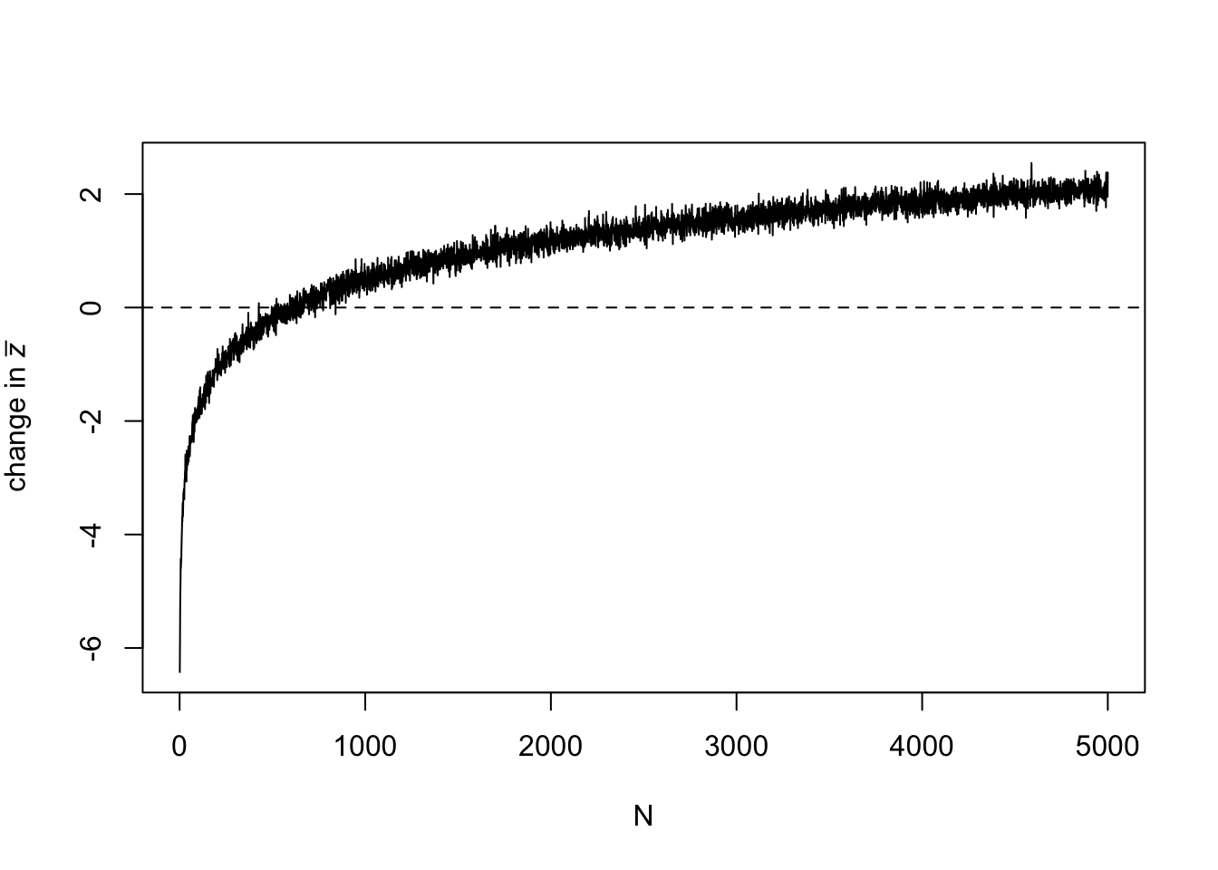
This plot shows that as \(N\) increases, \(\Delta \bar z\) flips from negative to positive. At low \(N\) there is cultural loss, at high \(N\) there is cultural gain. Note that there is some noise increasing the thickness of the line. This comes from the stochasticity of the simulation. The more generations we run, the less noise there is, but also the longer the simulation will take to run.
We can also run another pair of \(\alpha\) and \(\beta\) and compare the two lines on the same plot:
data_model9_2 <- DemographyModel2(N_max = 5000,
                                  alpha = 9,
                                  beta = 1,
                                  t_max = 100)

plot(1:length(data_model9_1), data_model9_1,
     type = 'l',
     ylab = expression("change in "*italic(bar("z"))),
     xlab = "N",
     col = "orange")

lines(data_model9_2, col = "royalblue")

abline(h = 0, lty = 2)

text(1300, 2,
     labels = expression("Simpler skill, "*alpha*"/"*beta*"=7"),
     col = "orange")
text(3000, -1.7,
     labels = expression("Complex skill, "*alpha*"/"*beta*"=9"),
     col = "royalblue")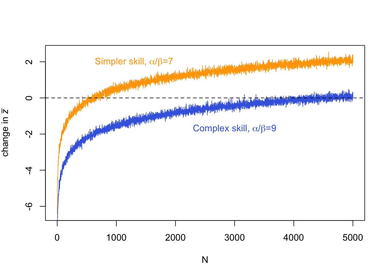
Here we have recreated Henrich’s (2004) Figure 3, comparing a ‘simple’ skill and a ‘complex’ skill. A simple skill is easier to learn than a complex skill, such that it has a smaller \(\alpha\) relative to \(\beta\) (remember, \(\alpha\) is copying error that always reduces skill, while \(\beta\) is inferences and guesses that sometimes leads to higher skill). The plot above shows that simpler skills require a smaller population size to be maintained (\(\Delta \bar z = 0\)) or improve (\(\Delta \bar z > 0\)) than more complex skills. This reflects the postulated Tasmanian case that we started with: when population sizes dropped when Tasmania became cut off from the mainland, complex skills like fishhooks were lost and never reinvented, while simpler skills remained. In the figure above, this would be like going from \(N = 5000\) to \(N = 1000\).
Summary
Cultural evolution occurs within populations of certain sizes and structures, and this population size and structure affects evolutionary dynamics. In previous models we have seen how population size can lead to the accidental loss of traits, which is a basic principle of genetic and cultural drift. Model 9 extended this basic finding to show how population size can determine whether there is cultural gain or cultural loss of a continuous cultural trait such as the skill required to make a hard-to-learn tool. Assuming that copying is imperfect, small populations are less able to maintain and accumulate cultural skill than large populations, even when every learner can identify and is attempting to learn from the highest skilled individual from the previous generation. Fewer learners means less chance that one of those learners will match or exceed that highest skilled individual from the previous generation. This effect of population size interacts with the ‘learnability’ and ‘improvability’ of the trait: more easily learned (lower \(\alpha\)) and more easily improved (higher \(\beta\)) traits require smaller populations to maintain and improve.
This model by Henrich (2004) has inspired a large body of subsequent models (e.g. Powell, Shennan & Thomas, 2009; Mesoudi 2011) and empirical research (e.g. Derex et al. 2013; Kline & Boyd 2010). These have extended the predictions of the model, and tested those predictions both in the laboratory and in real world datasets (see Derex & Mesoudi 2020). To be sure, population size is not the only determinant of cultural gains and losses. Even Henrich’s original model demonstrates this, given that learnability and improvability are also crucial. And more recent work has focused on population structure (e.g. social networks) rather than simply the number of individuals that are present. But there is no doubt that demography cannot be ignored when studying cultural evolution. Simulation models are often useful for studying demography, as complex population structures are difficult to implement in analytical models.
A few new programming techniques were used in Model 9. First, we introduced another continuous distribution, the gumbel distribution. Unlike the normal distribution used in Model 8, there are no built-in R functions for using the gumbel. We therefore had to write our own, and incorporate the rgumbel function into the simulation function. It is common practice to write user-defined functions for small routines and then call them within other functions. Indeed, it is often good practice, especially when the same set of lines of code are repeated in multiple places. Second, we used commands like expression, text and arrows to annotate plots. It is preferable to create plots entirely in R and then export the finished version (see Model 1 for how to do this), rather than export basic plots and annotate them in separate visual editing software or Powerpoint. Creating plots entirely in R is more reproducible because others can re-run your code and re-create your figures exactly. It also avoids loss of image resolution. Finally, we saw a few tricks to speed up code that takes a long time to run. Dataframes can be replaced with one-dimensional vectors when they are made up of just one variable. Means can be calculated by keeping a running total within a loop then dividing by the total number of data points once the loop has finished. Simplifying code as much as possible can often lead to significantly faster simulation runs, although try not to sacrifice code understandability in doing so.
Exercises
Try different values of \(\alpha\), \(\beta\) and \(N\) in DemographyModel to determine that, for given values of \(\alpha\) and \(\beta\), there is a threshold value of \(N\) above which there is cultural gain, and below which there is cultural loss.
Change DemographyModel so that there are two different population sizes, \(N_1\) and \(N_2\), both user-defined in the function call. For the first half of the generations, i.e. from \(t = 1\) to \(t = t_{max}/2\), the population size is \(N_1\). For the second half, i.e. from \(t = (t_{max}/2) + 1\) to \(t = t_{max}\), the population size is \(N_2\). For a given pair of \(\alpha\) and \(\beta\) values, pick an \(N_1\) that leads to cultural gain, and an \(N_2\) that leads to cultural loss. Run the simulation to see what happens. Is this a reasonable simulation of the purported ‘Tasmanian’ case described above and in Henrich (2004), where isolation due to rising sea levels caused a reduction in population size?
In Mesoudi (2011) I suggested that a simple way of making the Henrich (2004) model more realistic is to tie the copying error parameter \(\alpha\) to the mean skill level, \(\bar{z}\), in each generation. As skills become ever more complex, they should become harder to learn. If they are harder to learn, there will be more error in their transmission. Thus as \(\bar{z}\) increases over the generations, so should \(\alpha\). Modify the DemographyModel function to implement this additional assumption. As before, there should be a user-defined starting value of \(\alpha\). However, in each new timestep from \(t = 2\) onwards, \(\alpha\) should be multiplied by the mean skill level in the previous timestep (the latter is already being stored in the output dataframe). Run the simulation to see how this changes the dynamics of the model.
Analytic Appendix
Henrich’s (2004) model was analytical rather than simulation-based. We can use the analytical model to check our simulation results above, as well as additional things like calculate the exact \(N\) at which losses switch to gains for a given \(\alpha\) and \(\beta\).
As in the model above, we assume \(N\) individuals indexed by \(i\), with the \(i\)th individual possessing trait value \(z_i\). Each individual of each new generation draws a value from the gumbel distribution shown above, with mode \(z_h - \alpha\) and dispersion \(\beta\). As in the simulation model, we want to calculate \(\Delta \bar z\), the change in the mean trait value from one generation to the next.
The next generation mean trait value, \(\bar z'\), is given by:
\[ \bar z' = z_h + \Delta z_h \hspace{30 mm}(9.1)\]
Equation 9.1 says that the new mean trait value is the highest trait value in the previous generation, \(z_h\), plus any change in \(z_h\) as a result of imperfect copying. Henrich shows that the former can be approximated by:
\[ z_h = a + \beta (\epsilon + \ln(N)) \hspace{30 mm}(9.2)\]
where \(\epsilon\) is Euler’s constant, which is approximately 0.577.
The other term \(\Delta z_h\) is given by \(z_h' - z_h\). The new maximum value, \(z_h'\), is given by the mean of the gumbel distribution, \(a + \beta\epsilon\). The old maximum, \(z_h\), is given by \(a + \alpha\), as per the gumbel distribution figure above. Consequently:
\[ \Delta z_h = a + \beta\epsilon - a - \alpha = -\alpha + \beta\epsilon \hspace{30 mm}(9.3) \]
Substituting Equation 9.2 and 9.3 into Equation 9.1 gives:
\[ \bar z' = a + \beta (\epsilon + \ln(N)) -\alpha + \beta\epsilon \]
As \(\bar z' = \bar z + \Delta \bar z\) and \(a = \bar z - \beta \epsilon\),
\[ \Delta \bar z = \bar z - \beta \epsilon + \beta (\epsilon + \ln(N)) -\alpha + \beta\epsilon - \bar z \]
Simplifying, this gives:
\[ \Delta \bar z = -\alpha + \beta (\epsilon + \ln(N)) \hspace{30 mm}(9.4) \]
which is Henrich’s Equation 2. This says that, as we found in the simulation model, whether we see cultural gain or cultural loss depends on \(\alpha\), \(\beta\) and \(N\), but it also provides an exact relation between them.
By setting \(\Delta \bar z = 0\) and rearranging, we find that the equilibrium value of \(N\) at which there is neither gain nor loss, \(N^*\), is:
\[ N^* = e^{(\frac{\alpha}{\beta} - \epsilon)} \hspace{30 mm}(9.5)\]
and this is Henrich’s Equation 3. For the values \(\alpha = 30\) and \(\beta = 15\) used in the simulation model above, equation 9.5 gives \(N^* = 4.15\). When \(N\) is 4 or less we would expect cultural loss, and when \(N\) is 5 or more we would expect cultural gain. Try using the simulation model to confirm this.
Finally, we can use Equation 9.4 to recreate the figure above with the ‘simpler’ and ‘complex’ skills:
N_max <- 5000
delta_z <- rep(NA,N_max)

alpha <- 7
beta <- 1

for (N in 1:N_max) {

  delta_z[N] <- -alpha + beta * (-digamma(1) + log(N))

}

plot(1:length(delta_z), delta_z,
     type = 'l',
     ylab = expression("change in "*italic(bar("z"))),
     xlab = "N",
     col = "orange")

abline(h = 0, lty = 2)

alpha <- 9
beta <- 1

for (N in 1:N_max) {

  delta_z[N] <- -alpha + beta * (-digamma(1) + log(N))

}

lines(delta_z, col = "royalblue")

text(1300, 1.7,
     labels = expression("Simpler skill, "*alpha*"/"*beta*"=7"),
     col = "orange")
text(3000, -1.5,
     labels = expression("Complex skill, "*alpha*"/"*beta*"=9"),
     col = "royalblue")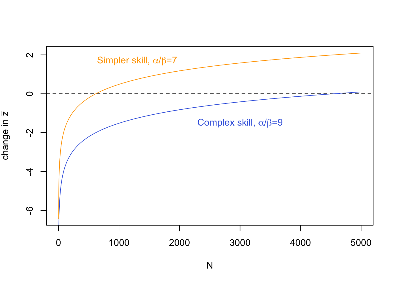
Note that Euler’s constant is provided in R as -digamma(1). Here we have reproduced the simulation figure above but in a fraction of the time, and with less noise.
References
Derex, M., Beugin, M. P., Godelle, B., & Raymond, M. (2013). Experimental evidence for the influence of group size on cultural complexity. Nature, 503(7476), 389-391.
Derex, M., & Mesoudi, A. (2020). Cumulative cultural evolution within evolving population structures. Trends in Cognitive Sciences, 24(8), 654-667.
Henrich, J. (2004). Demography and cultural evolution: How adaptive cultural processes can produce maladaptive losses - The Tasmanian case. American Antiquity, 69(2), 197-214.
Kline, M. A., & Boyd, R. (2010). Population size predicts technological complexity in Oceania. Proceedings of the Royal Society B: Biological Sciences, 277(1693), 2559-2564.
Mesoudi, A. (2011). Variable cultural acquisition costs constrain cumulative cultural evolution. PloS ONE, 6(3), e18239.
Powell, A., Shennan, S., & Thomas, M. G. (2009). Late Pleistocene demography and the appearance of modern human behavior. Science, 324(5932), 1298-1301.