Model 8: Blending inheritance
Introduction
When Darwin wrote The Origin of Species, it was typically thought that biological inheritance involved the blending of parental traits. For example, the offspring of a tall and a short individual would have intermediate height, the average (or blend) of its two parents. This presented a problem for Darwin’s theory, one which Darwin himself acknowledged. If traits blend together, then they are unlikely to persist for long enough for selection to act on them. All traits will quickly converge on a blended average, destroying the variation that is necessary for evolution.
This puzzle was resolved when Mendel’s famous pea plant experiments were rediscovered around the turn of the 20th century. These showed that genetic inheritance is actually particulate, not blending. This means that inheritance involves the passing of discrete particles of information - what became known as ‘genes’ - in an all-or-nothing fashion from parent to offspring. Some simple phenotypic traits, like Mendel’s pea plant varieties, show this directly. A white plant crossed with a purple plant gives rise to either a white or purple offspring, not a blend. Complex phenotypic traits like human height, which appear to ‘blend’ in offspring, are actually determined by many discrete genes.
A common objection to cultural evolution follows similar lines. Cultural traits, it is argued, are often continuous, and appear to blend in learners. Someone who grew up in Britain before moving to the States might have a blended ‘transatlantic’ accent. Someone with a liberal father and conservative mother might end up with moderate political views. If cultural inheritance is blending, then the same objection as that levied at Darwin above should also apply: variation will be rapidly lost, and evolution can’t operate. This is a common specific criticism of memetics, which assumes that there are discrete particles of inheritance analogous to genes.
One problem with this objection is that it is not at all clear that cultural inheritance is blending. We don’t know enough about how brains store and receive information to say with certainty that there is not a discrete, particulate inheritance system underlying what appears to be blending at the ‘phenotypic’ level, just like biological traits such as height appear to blend but are actually determined by an underlying particulate inheritance system. Another problem is that the objection cannot be true: there is huge cultural variation in the world that patently does exist, and upon which selection can and does act. So even if cultural inheritance is blending, perhaps some other feature of cultural evolution means that blending does not have the problematic consequences described above. Either way, it is worth exploring the case of blending inheritance with formal models to go beyond verbal arguments. Indeed, it was not until the formal population genetic models of R.A. Fisher and others in the early 20th century that Mendelian genetic inheritance and Darwinian evolution were definitively shown to be consistent with one another.
Model 8a: Blending inheritance
In Model 8a we will simulate blending cultural inheritance, inspired by a formal mathematical model presented by Boyd & Richerson (1985). We assume a population of \(N\) individuals. Each of these individuals possesses a value of a continuously varying cultural trait. While previous models have assumed discrete traits that can take on one of two forms (\(A\) or \(B\)), in this case we are modelling a trait that can take any value on a continuous scale. Many cultural traits are continuous, from handaxe length to political orientation.
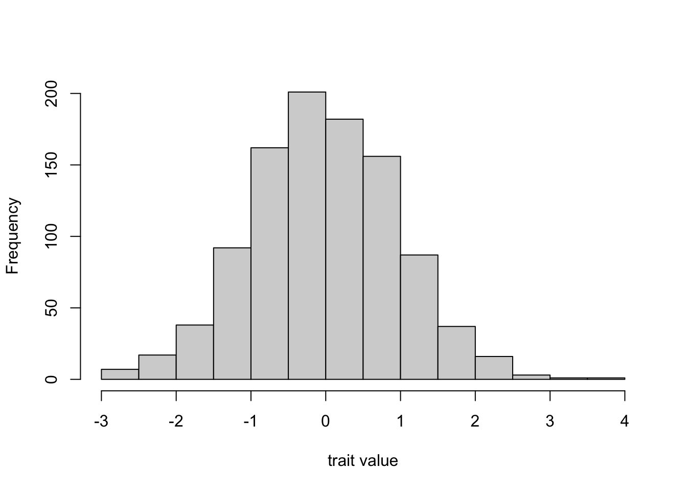
In the first generation / timestep, we assume that trait values are drawn randomly from a standard normal distribution. This is a symmetrical, bell-shaped distribution with mean 0 and standard deviation 1. It does not really matter what distribution or parameter values we use here. However, lots of naturally-occurring cultural traits are normally distributed. We might think of political orientation, where some people are on the extreme left or extreme right, and most are somewhere in the middle.
The rnorm command generates random numbers from this standard normal distribution, like this:
Hence this will be our initial distribution of trait values in the first generation. Then, in each new generation the \(N\) individuals are replaced with \(N\) new individuals. Each of these new agents picks \(n\) agents from the previous timestep at random and adopts the mean trait value of these \(n\) demonstrators. We assume that \(n > 1\) because we cannot really take a blended mean of a single trait value, and we assume that \(n \leq N\) because learners can only learn from a previous generation agent once.
In each timestep we track the mean trait value to see whether blending inheritance generates directional cultural change. We also track the variance of the trait across the entire population, in order to see whether and when blending inheritance destroys variation as per the objection above.
Below I have taken the skeleton of Model 1’s UnbiasedTransmission function, which has multiple independent runs and keeps track of and plots mean trait frequency, and adapted it to create a BlendingInheritance function. Examine the code before reading the explanation of the changes afterwards.
BlendingInheritance <- function (N, n, t_max, r_max) {

  # create a matrix for trait means with t_max rows and r_max columns,
  # fill with NAs, convert to dataframe
  trait_mean <- as.data.frame(matrix(NA, t_max, r_max))

  # purely cosmetic: rename the columns with run1, run2 etc.
  names(trait_mean) <- paste("run", 1:r_max, sep="")

  # same for holding trait variance
  trait_var <- as.data.frame(matrix(NA, t_max, r_max))
  names(trait_var) <- paste("run", 1:r_max, sep="")

  for (r in 1:r_max) {

    # create first generation, N random numbers from a standard normal distribution
    agent <- rnorm(N)

    # add first generation's mean to first row of column r
    trait_mean[1,r] <- mean(agent)

    # add first generation's variance to first row of column r
    trait_var[1,r] <- var(agent)

    for (t in 2:t_max) {

      # create matrix with N rows and n columns,
      # fill with traits from random members of agent
      m <- matrix(sample(agent, N*n, replace = TRUE), N, n)

      # create new generation by taking rowMeans, i.e. mean of n demonstrators,
      # to implement blending inheritance
      agent <- rowMeans(m)

      # get mean trait value and put it into output slot for this generation t and run r
      trait_mean[t,r] <- mean(agent)

      # get trait variance and put it into output slot for this generation t and run r
      trait_var[t,r] <- var(agent)

    }

  }

  # create two plots, one for means and one for variances
  par(mfrow=c(1,2)) # 1 row, 2 columns

  # plot a thick line for the mean mean of all runs
  plot(rowMeans(trait_mean),
       type = 'l',
       ylab = "trait mean",
       xlab = "generation",
       ylim = c(min(trait_mean,-1), max(trait_mean,1)),
       lwd = 3,
       main = paste("N = ", N, ", n = ", n, sep = ""))

  # add lines for each run, up to r_max
  for (r in 1:r_max) {
    lines(trait_mean[,r], type = 'l')
  }

  # plot a thick line for the mean variance across all runs
  plot(rowMeans(trait_var),
       type = 'l',
       ylab = "trait variance",
       xlab = "generation",
       ylim = c(0, max(trait_var)),
       lwd = 3,
       main = paste("N = ", N, ", n = ", n, sep = ""))

  # add lines for each run, up to r_max
  for (r in 1:r_max) {
    lines(trait_var[,r], type = 'l')
  }

  # export data from function
  list(final_agent = agent, mean = trait_mean, variance = trait_var)
}
First, rather than a single output dataframe, we create two, one called trait_mean to hold the mean trait value over all timesteps for all runs, and one called trait_variance to hold the variance of the trait over all timesteps and all runs. Then, in each run, we create an initial population which has \(N\) agents each with a trait value drawn randomly from a standard normal distribution using the rnorm command, as shown above. We then record the initial mean and variance in the appropriate slots of trait_mean and trait_variance respectively.
Within the timestep loop, we then create a matrix with \(N\) rows and \(n\) columns, and fill it with trait values from agents randomly selected using the sample command. Each row here represents a new agent, and each column of that row contains the trait values of \(n\) randomly chosen demonstrators, just like for horizontal transmission in Model 6c. We then use the rowMeans command to get the means of each row of this matrix. This is the blending inheritance rule. This mean (or blend) of the \(n\) demonstrators is put into the agent dataframe, over-writing the previous generation’s traits, and the new mean and variance are added to the output dataframes.
The subsequent plotting code now makes two plots side-by-side, one for the means and one for the variances. This is done with the par(mfrow([rows],[cols])) command, where [rows] is the number of rows and [cols] the number of columns. Here I’ve set one row and two columns. The actual plots use the same code as in previous models, with means across all runs plotted with thick lines and separate lines for each run. We do this twice, once for means, and once for variances.
Finally, rather than outputting a single dataframe, we now output three dataframes after the function is run: the final_agent dataframe, which allows us to explore the distribution of trait values at the very end of the simulation, and the trait_mean and trait_variance dataframes which contain the means and variances. We do this by exporting a list, which contains three dataframes.
Let’s run this function with a reasonably large \(N\) and small \(n\):
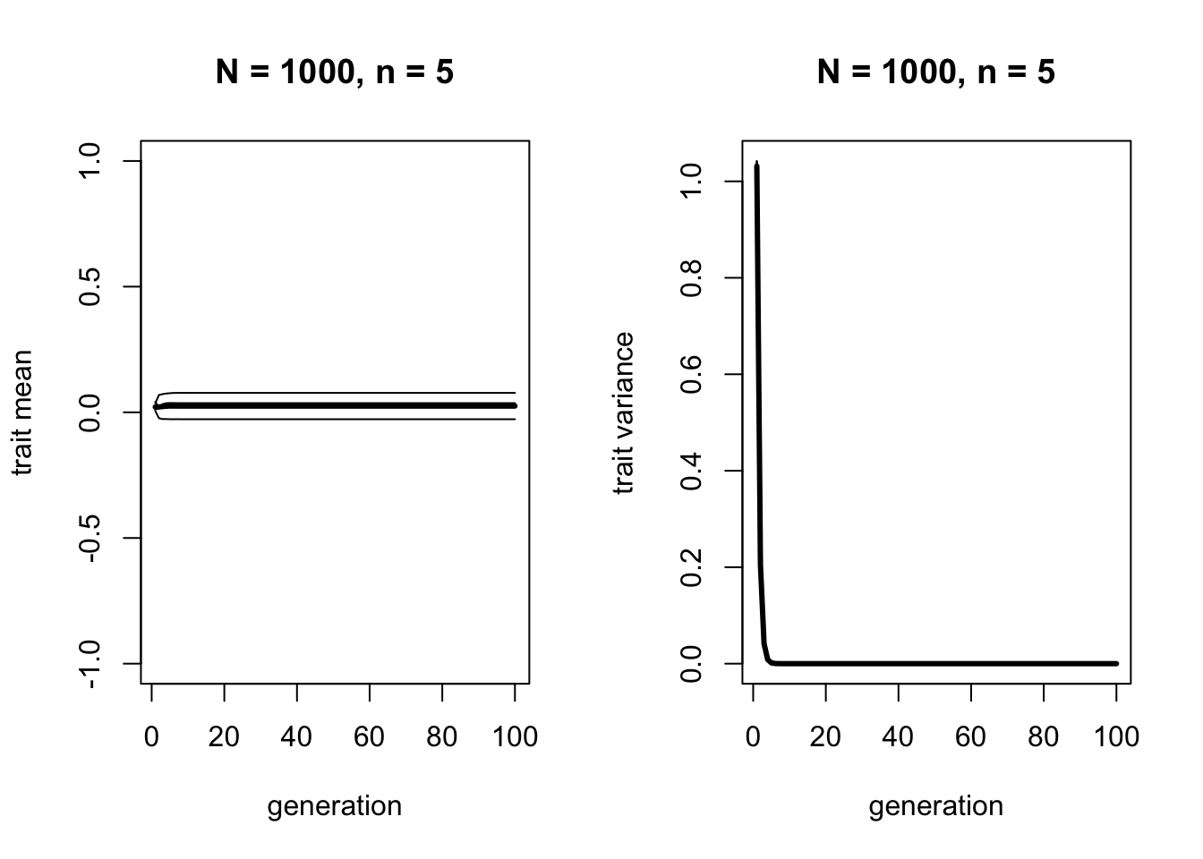
The left-hand plot shows that the mean across all runs remains at roughly 0, which is the mean of the initial standard normal distribution. Blending inheritance does not change mean trait value over time. It is non-directional, just like unbiased mutation or unbiased transmission. This is to be expected, as all we are doing is taking the mean of random draws from the previous generation’s trait distribution, which will be the same as the mean in the previous generation.
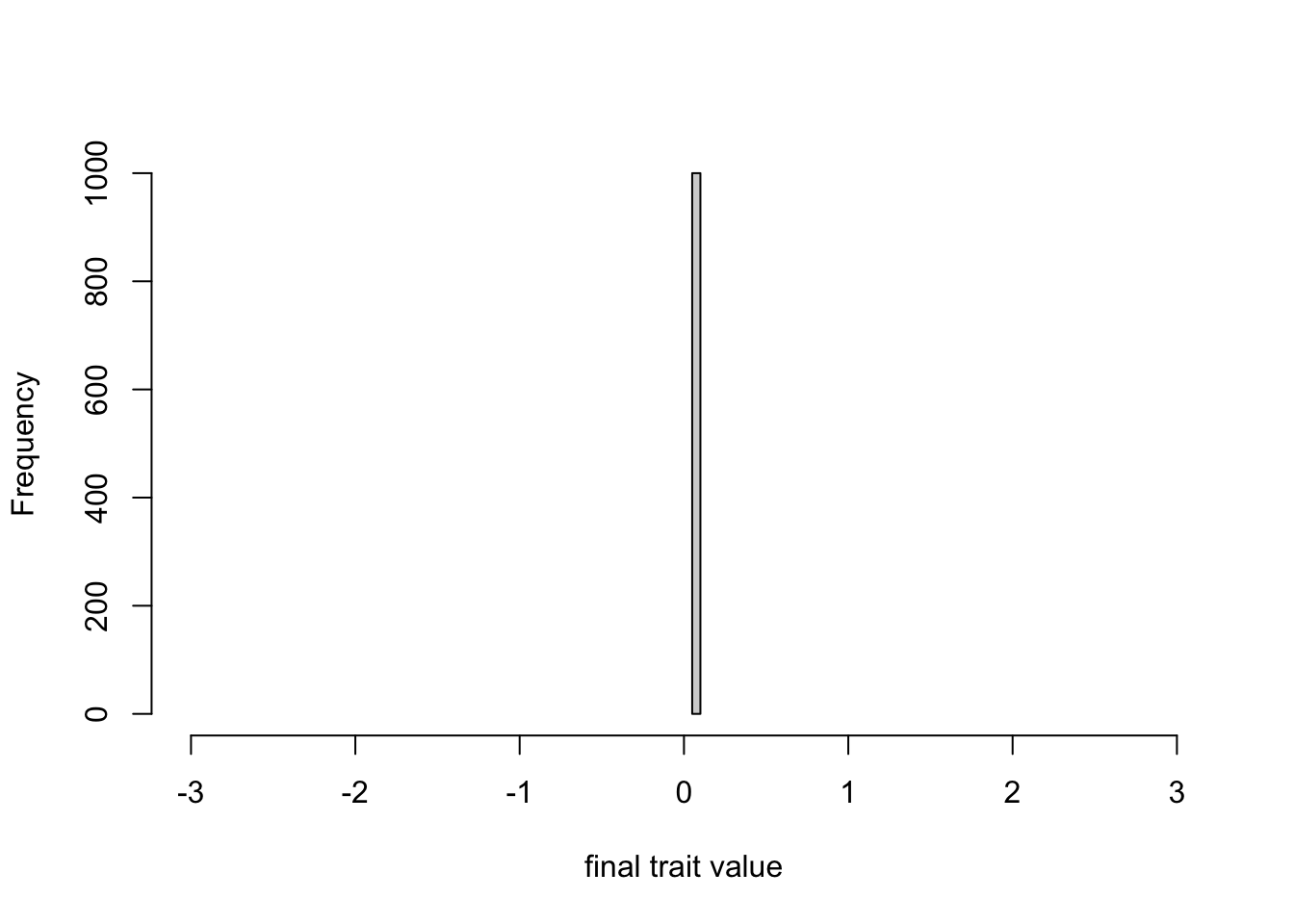
The right-hand plot shows that the variance quickly drops to zero. Again as we expected, blending inheritance acts to reduce variation to zero. We can confirm this by displaying some of the values of the final agent dataframe, to confirm that every agent has exactly the same trait:
## [1] 0.07734374 0.07734374 0.07734374 0.07734374 0.07734374 0.07734374## [1] 0.07734374 0.07734374 0.07734374 0.07734374 0.07734374 0.07734374We can also plot the final trait distribution on the same scale as the graph above showing the initial standard normal distribution, confirming that all of the initial variation has been lost.
Model 8b: Blending inheritance with mutation
All we have done so far is confirm the intuition that blending inheritance destroys variation, just as Darwin’s critics originally argued. If we assume that cultural traits in real life blend (which, as noted above, is far from certain), then it is hard to reconcile this conclusion with the observation of extensive cultural variation in real life.
However, we must remember that other aspects of cultural evolution may also differ from genetic evolution. Boyd & Richerson (1985) pointed out that blending inheritance is potentially problematic in biological evolution because rates of genetic mutation are low, and so cannot replenish the variation that blending inheritance destroys. Yet rates of cultural mutation may be much higher. In Model 8b we will follow their example and add unbiased cultural mutation, or copying error, to the blending inheritance model.
Previously we assumed that new agents could copy the traits of \(n\) agents from the previous timestep with no error, and then take the mean of these 100% accurate trait values. Now we assume that each of the \(n\) cultural traits are copied with some error, similar to unbiased cultural mutation in Model 2. So before the blended mean is taken, random error is added to each copied trait value.
We do this by again using the rnorm command to draw randomly from a normal distribution. This time, the normal distribution has a mean of the copied trait values, which are stored in the m matrix, and the random error or deviation is introduced to each one using a new parameter \(e\). This is the variance of this normal distribution. The larger is \(e\), the more error or mutation there is in the estimates of each of the \(n\) traits. Note that each of the \(n\) copied traits are subject to independent error. Some might be copied quite faithfully, others less faithfully. Blending inheritance then proceeds as before, but now it is the mean of the modified trait values.
The following code modifies the BlendingInheritance function above by adding a parameter \(e\), and adding a line after the trait copying in which the m matrix is modified according to \(e\). Note that because \(e\) is the variance of the error distribution (following Boyd & Richerson 1985), and the rnorm function takes a standard deviation, we need to give the function the square root of \(e\). We also add \(e\) to the plot title.
BlendingInheritance <- function (N, n, e, t_max, r_max) {

  # create a matrix for trait means with t_max rows and r_max columns,
  # fill with NAs, convert to dataframe
  trait_mean <- as.data.frame(matrix(NA, t_max, r_max))

  # purely cosmetic: rename the columns with run1, run2 etc.
  names(trait_mean) <- paste("run", 1:r_max, sep="")

  # same for holding trait variance
  trait_var <- as.data.frame(matrix(NA, t_max, r_max))
  names(trait_var) <- paste("run", 1:r_max, sep="")

  for (r in 1:r_max) {

    # create first generation, N random numbers from a standard normal distribution
    agent <- rnorm(N)

    # add first generation's mean to first row of column r
    trait_mean[1,r] <- mean(agent)

    # add first generation's variance to first row of column r
    trait_var[1,r] <- var(agent)

    for (t in 2:t_max) {

      # create matrix with N rows and n columns,
      # fill with traits from random members of agent
      m <- matrix(sample(agent, N*n, replace = TRUE), N, n)

      # add random error to each demonstrator value, with variance e
      m <- matrix(rnorm(N*n, mean = m, sd = sqrt(e)), N, n)

      # create new generation by taking rowMeans, i.e. mean of n demonstrators,
      # to implement blending inheritance
      agent <- rowMeans(m)

      # get mean trait value and put it into output slot for this generation t and run r
      trait_mean[t,r] <- mean(agent)

      # get trait variance and put it into output slot for this generation t and run r
      trait_var[t,r] <- var(agent)

    }

  }

  # create two plots, one for means one for variances
  par(mfrow=c(1,2)) # 1 row, 2 columns

  # plot a thick line for the mean mean of all runs
  plot(rowMeans(trait_mean),
       type = 'l',
       ylab = "trait mean",
       xlab = "generation",
       ylim = c(min(trait_mean,-1), max(trait_mean,1)),
       lwd = 3,
       main = paste("N = ", N, ", n = ", n, ", e = ", e, sep = ""))

  # add lines for each run, up to r_max
  for (r in 1:r_max) {
    lines(trait_mean[,r], type = 'l')
  }

  # plot a thick line for the mean variance across all runs
  plot(rowMeans(trait_var),
       type = 'l',
       ylab = "trait variance",
       xlab = "generation",
       ylim = c(0, max(trait_var)),
       lwd = 3,
       main = paste("N = ", N, ", n = ", n, ", e = ", e, sep = ""))

  # add lines for each run, up to r_max
  for (r in 1:r_max) {
    lines(trait_var[,r], type = 'l')
  }

  # export data from function
  list(final_agent = agent, mean = trait_mean, variance = trait_var)
}
First we can run this code with \(e = 0\), to confirm that this matches the original function which had no error.
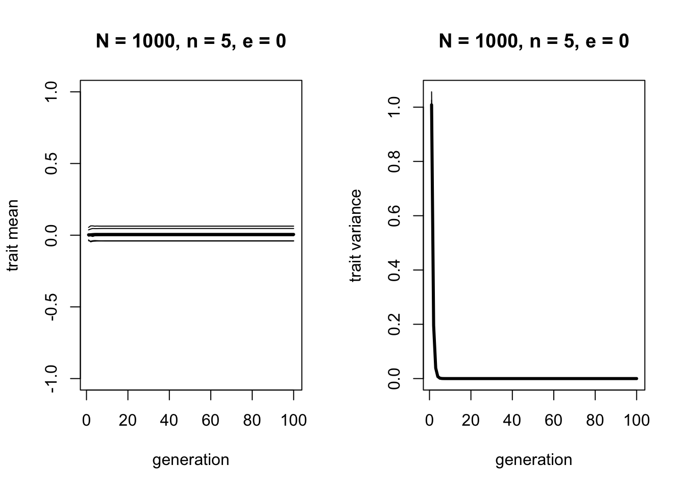
As before, the mean does not change, and variation decreases to zero. Now let’s increase \(e\):
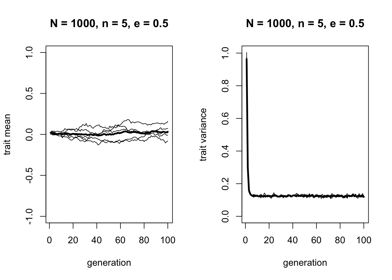
There are two changes here. First, in the left hand plot we can see that while the mean of the mean trait value still does not change and remains around zero, there is more variation around this line in the different runs. Consistent with this, the right hand plot shows that while the variance still drops, it does not drop to zero. For \(n = 5\) and \(e = 0.5\), the variance converges on around 0.125. We can see this more exactly by displaying the mean variances for each run over the last 50 timesteps (to avoid the initial value from skewing the estimate):
##      run1      run2      run3      run4      run5
## 0.1237358 0.1237820 0.1243846 0.1247881 0.1248948
Try playing around with \(n\) and \(e\) to show that the equilibrium amount of variance increases as \(e\) increases and as \(n\) decreases. In the analytical appendix we will see how to calculate this equilibrium value from \(n\) and \(e\).
Finally, we can plot the trait distribution in the final generation.
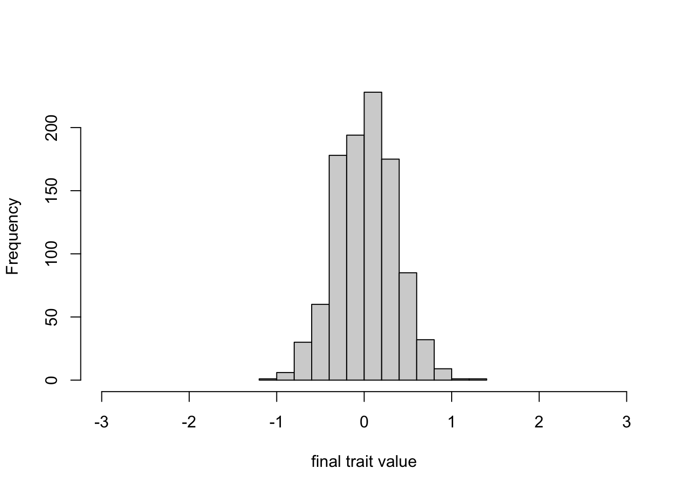
While the first plot above showed that the initial distribution ranged from around -3 to 3, this final distribution ranges from around -1 to 1. So while there is less variation than in the first generation, there is still variation, and it still resembles a normal distribution.
Summary
A common objection to cultural evolution is that cultural inheritance blends different traits together, destroying the variation that is necessary for evolution to operate. While the claim that cultural inheritance is blending can be contested, and obviously it is not the case that there is no cultural variation in the real world, we can still use formal models to explore these claims.
Model 8a confirmed that blending inheritance destroys variation, as expected. However, Model 8b showed that this can be countered by cultural mutation. While genetic mutation is very infrequent, cultural mutation is probably much more common. People typically misremember facts, distort stories, and modify tools as they attempt to copy others. So even if cultural inheritance does take the form of blending, it is quite plausible that cultural mutation is potent enough to re-introduce variation that blending destroys. While we did not model this here, a similar argument can be made for cultural selection. While natural selection tends to be weak, cultural selection may be much stronger. So even if blending inheritance reduces variation, strong cultural selection can still act before the variation is depleted.
There are also a few programming innovations introduced in Model 8. We modelled a continuously varying cultural trait, rather than a discrete trait that could take one of two values as in previous models. This means we had to specify the distribution of the continuous trait, and track the mean and variance of that distribution, rather than a trait frequency. We used the command rnorm to draw random trait values from a normal distribution in order to create the initial generation’s trait values. We also used rnorm to simulate random error or mutation in the transmission of the continuous trait. The copied trait value is set as the mean of the normal distribution, with the error around this value set by the standard deviation (or variance) of the normal distribution. Finally, we saw how to create two plots side-by-side using the par(mfrow=c([rows],[cols])) command.
Exercises
Try different values of \(N\) and \(n\) in BlendingInheritance to see how blending inheritance reduces variation to zero whenever \(n>1\).
Try different values of \(n\) and \(e\) to show that the former increases the blending effect, and the latter reduces it.
Forgetting about blending for now, combine Model 3 and Model 8 to create a function that models selection (i.e. directly biased transmission, from Model 3) on a continuous cultural trait (as implemented in Model 8). Instead of \(s\) being the probability of switching to trait \(A\) upon encountering a demonstrator with that trait as in Model 3, instead assume that there is a particular value of the continuous trait that is particularly attractive, memorable or intuitive. Allow the user to set this value when calling the function. For example, it might be zero (the mean of the starting normal distribution), or a different value (say +3, or -2). Then, each agent picks a random member of the previous generation, and if the demonstrator’s value is closer to the favoured value, and with probability \(s\) (as in Model 3), then the copying agent adopts the demonstrator’s value. Otherwise they do not copy and retain their previous value. Run the simulation to see what happens to the mean and variance over time.
Modify the function you just created to allow selection for two different trait values, rather than just one. Now, with probability \(s\), each agent picks a random demonstrator from the previous generation, and if the demonstrator’s value is closer to either of the two favoured values, then the agent adopts that closest value. Run the simulation to see what happens to the mean and variance over time.
Add blending inheritance to the function you just created, using the code from Model 8. Use a parameter to switch blending on (e.g. blend = TRUE) or off (e.g. blend = FALSE). With \(e=0\), explore under what conditions selection (via \(s\)) prevents blending from destroying variation.
Analytic Appendix
The simulation model presented above recreates an analytical model presented in Chapter 3 of Boyd & Richerson (1985), and we replicate their conclusions. They also include assortative transmission, which has a similar effect to mutation: if the \(n\) demonstrators have similar cultural traits, then blending inheritance is less effective at reducing variation. Box 3.22 in Boyd & Richerson (1985) provides a proof that the mean trait value after blending inheritance, \(\bar{X}'\), equals the mean trait value before blending inheritance, \(\bar{X}\). Their equation 3.28 does the same for variance under the assumption of transmission error, where variance after blending inheritance, \(V'\), is given by:
\[ V' = (1/n)(V + \bar{E}) \hspace{30 mm}(8.1)\]
where \(\bar{E}\) is the mean value of \(e\) across all demonstrators, and \(e\) is defined as in the simulation model. Because \(e\) is a constant across all demonstrators, and the errors are independent, \(\bar{E}\) will equal \(e\). To get the equilibrium variance, \(\hat{V}\), we can set \(V' = V\) in the above equation and rearrange to find:
\[ \hat{V} = \frac{e}{n-1} \hspace{30 mm}(8.2)\]
For the \(e = 0.5\) and \(n = 5\) simulated above, this gives \(\hat{V} = 0.5 / 4 = 0.125\), as was found in the simulation. This equation confirms that the variation remaining after blending inheritance increases with \(e\) and decreases with \(n\).