Model 17: Reinforcement learning
Introduction
It’s fair to say that the field of cultural evolution focuses far more on social learning (learning from others) than individual learning (learning on one’s own). While we have modelled several different types of social learning (direct bias, indirect bias, conformity, vertical transmission etc.), individual learning has taken relatively simple forms, such as the cultural mutation of Model 2. Here individuals invent a new cultural trait or switch to a different cultural trait with a certain probability. This is a reasonable starting point but can be much improved to give a more psychologically informed model of individual learning. After all, without new variation introduced by individual learning, cultural evolution cannot occur, so individual learning deserves more attention.
Model 17 will implement reinforcement learning, a popular method of modelling individual learning across several disciplines. Reinforcement learning has its roots in psychology, where early behaviourists like Edward Thorndyke, Ivan Pavlov and BF Skinner argued that behaviours which get rewarded (or ‘reinforced’) increase in frequency, while behaviours that are unrewarded are performed less often. More recently, reinforcement learning has become popular in machine learning and artificial intelligence (Sutton & Barto 2018). In these fields reinforcement learning is defined as learning from the environment what actions or choices maximise some numerical reward. This reward might be points in a game, money in a transaction, even happiness if we are willing to assign it a numerical value. Researchers studying reinforcement learning devise algorithms - models, essentially - that can achieve this maximisation.
In the field of cultural evolution, reinforcement learning models have been used in lab experiments to model participants’ choices in decision-making tasks, combined with the social learning biases that we have already come across (e.g. McElreath et al. 2008; Barrett et al. 2017; Toyokawa et al. 2019; Deffner et al. 2020). In Model 17 we will recreate simple versions of these studies’ models to see how to simulate individual learning as reinforcement learning and how to combine it with social learning.
Also, in a ‘Statistical Appendix’ we will see how to retrieve parameters of our reinforcement-plus-social-learning models from simulation data. In other words, we run our agent-based simulation of reinforcement and social learning with various known parameters, such as a probability \(s = 0.3\) that an agent engages in social learning rather than reinforcement learning. This gives us our familiar output dataframe containing all the traits of all agents over all trials. We then feed this output dataframe into the statistical modelling platform Stan, without the original parameter values, to try to retrieve those parameter values. In the example above we would hope to obtain \(s = 0.3\) or thereabouts, rather than \(s = 0.1\) or \(s = 0.9\). This might seem somewhat pointless with simulated data when we already know what the parameters were. But in experiments and analyses of real world data we won’t know in advance what real people’s tendencies to engage in social learning are, or their propensity for conformity, etc. By testing statistical analyses on agent-based simulation data, we can confirm that our statistical methods adequately estimate such parameters. This is another valuable use for agent-based models.
Model 17a: Reinforcement learning with a single agent
Before simulating multiple agents who can potentially learn from one another, we start with a single agent. This is all we need for individual learning and will help to better understand how reinforcement learning works.
In models of reinforcement learning agents typically face what is known as a multi-armed or \(k\)-armed bandit task. A ‘one-armed bandit’ is a slot machine like you would find in a casino. You pull the lever and hope to get a reward. A \(k\)-armed bandit is a set of \(k\) of these slot machines. On each trial the agent pulls one of the \(k\) arms and gets a reward. While all arms give rewards, they differ in the average size of the reward. However, the agent doesn’t know these average rewards in advance. The agent’s task is therefore to learn which of the \(k\) arms gives the highest average reward by pulling the arms and observing the rewards.
To make things difficult, there is random noise in the exact size of the reward received on each trial. The agent can’t just try each arm and immediately know which is best, they must learn which is best over successive trials each of which gives noisy data.
We can implement this by assuming that each arm’s reward is drawn randomly from a normal distribution with a different mean for each arm and a common standard deviation \(\sigma\). We will use a simplified version of the reward environment implemented in an experiment by Deffner et al. (2020). They had \(k = 4\) arms. One arm gave a higher mean reward than the other three, which all had the same mean reward. We assume that the optimal arm (arm 4) has a mean reward of 13 points, and the others (arms 1-3) have a mean reward of 10 points. All arms have a standard deviation \(\sigma = 1.5\). Let’s plot these reward distributions:
# define parameters of the 4-armed bandit task
arm_means <- c(10,10,10,13)
arm_sd <- 1.5

# empty plot
plot(NA,
     ylab = "probability density",
     xlab = "reward",
     type = 'n',
     bty='l',
     xlim = c(4, 20),
     ylim = c(0, 0.3))

# plot each arm's normally distributed reward
x <- seq(-10, 100, 0.1)
polygon(x, dnorm(x, arm_means[1], arm_sd), col = adjustcolor("royalblue", alpha.f = 0.2))
text(10, 0.29, "arms 1-3")
polygon(x, dnorm(x, arm_means[4], arm_sd), col = adjustcolor("orange", alpha.f = 0.2))
text(13, 0.29, "arm 4")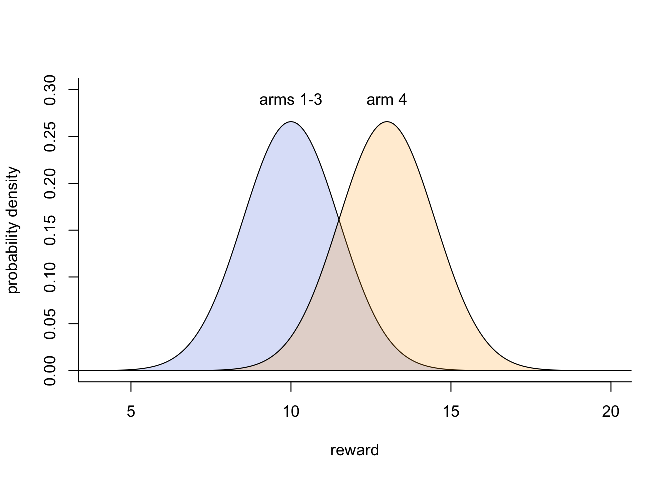
While arm 4 gives a higher reward on average, there is overlap with the other three arms’ reward distributions. This is made more concrete by picking 10 values from each arm’s reward distribution:
m <- matrix(NA, nrow = 4, ncol = 10,
            dimnames = list(c("arm1","arm2","arm3","arm4"), NULL))

for (i in 1:4) m[i,] <- round(rnorm(10, arm_means[i], arm_sd))

m
## [,1] [,2] [,3] [,4] [,5] [,6] [,7] [,8] [,9] [,10]
## arm1 11 10 12 10 12 11 11 11 10 10
## arm2 9 6 8 9 9 11 12 6 8 7
## arm3 11 11 9 10 10 8 11 11 9 10
## arm4 13 13 12 12 12 12 16 16 13 12Think of each of the 10 columns as an agent trying all four arms once to see which gives the highest reward. While most of the 10 columns will show that arm 4 gives a higher reward than the other arms, some won’t. This is the challenge that the agent faces. Over successive trials, they must maximise rewards by picking from the arm that gives the highest mean reward without knowing which arm does this in advance, and with noisy feedback from the environment. (NB the parameter \(\sigma\) controls this uncertainty; try increasing it to \(\sigma = 3\) and rerunning the two code chunks above, to see how the task becomes even more difficult.)
A fundamental problem which arises in tasks such as the \(k\)-armed bandit is an exploitation vs exploration tradeoff. Imagine an agent picks each of the above four arms once on four successive trials. There is a chance that arm 4 gives the highest reward, but it’s far from certain (in how many of the 10 columns in the rewards output above does arm 4 give the single highest reward?). Imagine instead that arm 2 gives the highest reward. A highly exploitative agent will proceed to pick (‘exploit’) arm 2 until the end of the simulation, believing (falsely) that arm 2 maximises its rewards. At the other extreme, a highly exploratory agent will continue to try all of the other arms to gain as much information about the reward distributions as possible. Both agents lose out: the exploitative agent is losing out on the rewards it would have got if it had explored more and discovered that arm 4 is actually the best, while the exploratory agent is losing out because it never settles on arm 4, continuing to pick arms 1-3 until the end.
What is needed is an algorithm that balances exploitation and exploration to explore enough to find the best option, but not too much so that the best option is exploited as much as possible. That’s what we’ll implement in Model 17a.
First we need to numerically represent the agent’s estimate of the value of each arm. These estimates are called Q values (or sometimes ‘attractions’, denoted \(A\)). The agent has one Q value for each arm. Q values can take any value - fractions, zeroes, negative numbers, etc. - as long as they numerically specify the relative value of each action.
We create a variable Q_values to hold the agent’s Q values for each arm on the current trial:
# for storing Q values for 4 arms on current trial
Q_values <- rep(0, 4)
names(Q_values) <- paste("arm", 1:4, sep="")

Q_values
## arm1 arm2 arm3 arm4
## 0 0 0 0On the first trial (\(t = 1\)) we’ll set each Q value to zero, as shown above. This indicates that the agent has no initial preference for any of the arms. If we had prior knowledge about the arms we might set different values, but for now equal preferences is a reasonable assumption.
Now we convert these values into probabilities, specifying the probability that the agent chooses each arm on the next trial. This is where the exploitation-exploration trade-off is addressed. We use what is called a ‘softmax’ function, which converts any set of values into probabilities that sum to one (as probabilities must) and weights the probabilities according to those values. The higher the relative value, the higher the relative probability.
The softmax function contains a parameter \(\beta\), often called ‘inverse temperature’, that determines how exploitative the agent is (sometimes expressed as how ‘greedy’ the agent is). When \(\beta = 0\), arms are chosen entirely at random with no influence of the Q values. This is super exploratory, as the agent continues to choose all arms irrespective of observed rewards. As \(\beta\) increases, there is a higher probability of picking the arm with the highest Q value. This is increasingly exploitative (or ‘greedy’). When \(\beta\) is very large then only the arm that currently has the highest Q value will be chosen, even if other arms might actually be better.
Mathematically, the softmax function looks like this:
\[ p_i = \frac{e^{\beta Q_i}}{\sum_{j=1} ^k {e^{\beta Q_j}}} \hspace{30 mm}(17.1)\]
On the left hand side \(p_i\) means the probability of choosing arm \(i\). This is equal to the exponential of the product of the parameter \(\beta\) and the \(Q\) value of arm \(i\), divided by the sum of this value for all arms (\(Q_j\) for \(j = 1\) to \(j = k\), where \(k = 4\) in our case).
Some code will help to understand this equation. The softmax function can easily be written in R as follows, defining \(\beta = 0\) for now:
## arm1 arm2 arm3 arm4
## 0.25 0.25 0.25 0.25
Given that our initial Q values are all zero, each arm has an equal probability of being chosen. \(\beta\) is irrelevant here as no arm has the highest reward yet. Let’s try a different set of Q values, representing a hypothetical set of four trials, one per arm, like one of the 10 columns in the matrix above:
## arm1 arm2 arm3 arm4
## 0.25 0.25 0.25 0.25
Because \(\beta = 0\), the new Q values make no difference. The agent still picks each arm with equal probability. Now we increase \(\beta\) to 0.3 (rounding the display to 2 decimal places for ease of reading using the round function):
## arm1 arm2 arm3 arm4
## 0.13 0.44 0.10 0.33
Now arm 2 is more likely to be chosen, given that it has the highest reward. But it’s still possible that the other arms are chosen, particularly arm 4 which has an only slightly lower reward than arm 2. This seems like a good value of \(\beta\) to balance exploitation and exploration: the currently highest valued arm is most likely to be chosen, but there is a chance of exploring other arms, particularly other relatively high-scoring arms.
To check this, we increase \(\beta\) to a much higher value:
## arm1 arm2 arm3 arm4
## 0.00 0.99 0.00 0.01
It’s now almost certain that arm 2 is chosen. This \(\beta\) value is probably too large. It will greedily exploit arm 2 without ever exploring the other arms, and never discover that arm 4 is better.
For now we’ll revert to our initial all-equal Q values and a reasonable \(\beta = 0.3\). Our agent stores the softmax probabilities in probs then uses this in sample to choose one of the four arms. This choice is stored in choice.
Q_values[1:4] <- rep(0,4)
beta <- 0.3

probs <- exp(beta * Q_values) / sum(exp(beta * Q_values))

choice <- sample(1:4, 1, prob = probs)
choice
## [1] 3The arm number above will vary on different simulations, given that it is essentially a random choice. Next the agent pulls the chosen arm and gets a reward, using the command rnorm to pick a random number from one of the normal distributions specified above. Note that we round the reward to the nearest integer to avoid unwieldy decimals.
## [1] 13This reward will also vary on different simulations, as it’s a random draw from a normal distribution with a randomly selected mean.
Finally, the agent updates its Q values given the reward. The extent to which Q values are updated is controlled by a second parameter, \(\alpha\), which ranges from 0 to 1. When \(\alpha = 0\) there is no updating and the reward has no effect on Q values. When \(\alpha = 1\) the Q value for the rewarded arm increases by the full reward amount. When \(0 < \alpha < 1\) the Q value for the rewarded arm increases by a proportion \(\alpha\) of the reward. There is again a trade-off here. Obviously \(\alpha = 0\) is no good because the agent is not learning. However, if \(\alpha\) is too large then the agent can prematurely focus on an arm that gives a high reward early on, without exploring other arms.
The following code updates the Q values according to \(\alpha = 0.7\) and the reward:
## arm1 arm2 arm3 arm4
##  0.0  0.0  9.1  0.0
You can see that the chosen arm’s Q value has increased by \(\alpha\) times the reward shown above. The other arms remain zero.
We then repeat these steps (get probabilities, make choice, get reward, update Q values) over each of \(t_{max} = 100\) timesteps. But let’s add a final twist. Every 25 timesteps we will change which arm gives the higher reward. This lets us see whether our reinforcement algorithm can handle environmental change, rather than blindly sticking with arm 4 even after it is no longer optimal.
The following function RL_single does all this, using a dataframe output to store the Q values, choice and reward for each trial. For simplicity, we hard code the number of arms (\(k\)), the arm means and standard deviations, and the number of timesteps (\(t_{max}\)) rather than making them user-defined variables.
RL_single <- function(alpha, beta) {

  # set up arm rewards
  arm_means <- data.frame(p1 = c(10,10,10,13),
                          p2 = c(10,13,10,10),
                          p3 = c(13,10,10,10),
                          p4 = c(10,10,13,10))
  arm_sd <- 1.5

  # for storing Q values for 4 arms on current trial, initially all zero
  Q_values <- rep(0, 4)

  # for storing Q values, choices, rewards per trial
  output <- as.data.frame(matrix(NA, 100, 6))
  names(output) <- c(paste("arm", 1:4, sep=""), "choice", "reward")

  # t-loop
  for (t in 1:100) {

    # get softmax probabilities from Q_values and beta
    probs <- exp(beta * Q_values) / sum(exp(beta * Q_values))

    # choose an arm based on probs
    choice <- sample(1:4, 1, prob = probs)

    # get reward, given current time period
    if (t <= 25) reward <- round(rnorm(1, mean = arm_means$p1[choice], sd = arm_sd))
    if (t > 25 & t <= 50) reward <- round(rnorm(1, mean = arm_means$p2[choice], sd = arm_sd))
    if (t > 50 & t <= 75) reward <- round(rnorm(1, mean = arm_means$p3[choice], sd = arm_sd))
    if (t > 75) reward <- round(rnorm(1, mean = arm_means$p4[choice], sd = arm_sd))

    # update Q_values for choice based on reward and alpha
    Q_values[choice] <- Q_values[choice] + alpha * (reward - Q_values[choice])

    # store all in output dataframe
    output[t,1:4] <- Q_values
    output$choice[t] <- choice
    output$reward[t] <- reward

  }

  # record whether correct
  output$correct <- output$choice == c(rep(4,25),rep(2,25),rep(1,25),rep(3,25))

  # export output dataframe
  output

}
The core code regarding Q values, probabilities and choices is as it was earlier. However, instead of a single set of arm_rewards, we now create a dataframe with the different rewards for the four time periods (p1 to p4). These are then used later to calculate the reward given the current time period. The output dataframe records each Q value, choice and reward for each timestep. After the t-loop, a variable is created within output called correct which records whether the agent picked the optimal arm for that timestep.
Here is one run of RL_single with the parameter values from above, showing the first period of 25 timesteps when arm 4 is optimal:
##        arm1      arm2      arm3 arm4 choice reward correct
## 1  0.000000  6.300000  0.000000  0.0      2      9   FALSE
## 2  0.000000  6.300000  5.600000  0.0      3      8   FALSE
## 3  0.000000  6.300000  6.580000  0.0      3      7   FALSE
## 4  0.000000  9.590000  6.580000  0.0      2     11   FALSE
## 5  0.000000  9.590000  8.974000  0.0      3     10   FALSE
## 6  0.000000  9.590000  8.992200  0.0      3      9   FALSE
## 7  0.000000  9.590000  8.997660  0.0      3      9   FALSE
## 8  0.000000  9.590000  8.299298  0.0      3      8   FALSE
## 9  0.000000  9.590000  8.089789  0.0      3      8   FALSE
## 10 0.000000  9.590000  8.726937  0.0      3      9   FALSE
## 11 0.000000  9.590000  8.726937  8.4      4     12    TRUE
## 12 0.000000  9.590000  9.618081  8.4      3     10   FALSE
## 13 0.000000  9.590000  8.485424  8.4      3      8   FALSE
## 14 0.000000  9.877000  8.485424  8.4      2     10   FALSE
## 15 0.000000 11.363100  8.485424  8.4      2     12   FALSE
## 16 0.000000 10.408930  8.485424  8.4      2     10   FALSE
## 17 5.600000 10.408930  8.485424  8.4      1      8   FALSE
## 18 9.380000 10.408930  8.485424  8.4      1     11   FALSE
## 19 9.114000 10.408930  8.485424  8.4      1      9   FALSE
## 20 9.734200 10.408930  8.485424  8.4      1     10   FALSE
## 21 9.920260 10.408930  8.485424  8.4      1     10   FALSE
## 22 9.920260  8.722679  8.485424  8.4      2      8   FALSE
## 23 8.576078  8.722679  8.485424  8.4      1      8   FALSE
## 24 8.576078  8.722679  8.845627  8.4      3      9   FALSE
## 25 8.576078  8.722679 11.053688  8.4      3     12   FALSE
Each run will be different, but you can see the Q values gradually updating over these 25 timesteps. Perhaps arm 4 ends the period with the highest Q value. Perhaps not. Possibly not all arms got explored. The task is difficult and this learning algorithm is not perfect. But some learning is occurring. What about the final 25 timesteps, where arm 3 is optimal?
##          arm1     arm2      arm3     arm4 choice reward correct
## 76  14.701333 11.00427  9.774522 7.673512      2     12   FALSE
## 77  10.010400 11.00427  9.774522 7.673512      1      8   FALSE
## 78  10.010400 11.00427 12.032357 7.673512      3     13    TRUE
## 79  10.010400 11.00128 12.032357 7.673512      2     11   FALSE
## 80  10.010400 11.00128 12.709707 7.673512      3     13    TRUE
## 81  12.103120 11.00128 12.709707 7.673512      1     13   FALSE
## 82  12.103120 10.30038 12.709707 7.673512      2     10   FALSE
## 83   9.230936 10.30038 12.709707 7.673512      1      8   FALSE
## 84   9.230936 10.30038 12.212912 7.673512      3     12    TRUE
## 85   9.230936 10.09012 12.212912 7.673512      2     10   FALSE
## 86   9.230936 10.09012 12.063874 7.673512      3     12    TRUE
## 87  10.469281 10.09012 12.063874 7.673512      1     11   FALSE
## 88  10.469281 10.09012 12.063874 7.902054      4      8   FALSE
## 89  10.469281 10.02703 12.063874 7.902054      2     10   FALSE
## 90  12.240784 10.02703 12.063874 7.902054      1     13   FALSE
## 91  10.672235 10.02703 12.063874 7.902054      1     10   FALSE
## 92  10.672235 10.00811 12.063874 7.902054      2     10   FALSE
## 93  10.672235 10.00811 12.063874 7.970616      4      8   FALSE
## 94  10.672235 10.00811 12.719162 7.970616      3     13    TRUE
## 95  10.201671 10.00811 12.719162 7.970616      1     10   FALSE
## 96  10.201671 10.00811 15.015749 7.970616      3     16    TRUE
## 97  10.201671 10.00811 15.704725 7.970616      3     16    TRUE
## 98  10.201671 10.00811 15.704725 8.691185      4      9   FALSE
## 99  10.201671 10.00811 14.511417 8.691185      3     14    TRUE
## 100 10.201671 10.00811 13.453425 8.691185      3     13    TRUE
Again, each run will be different, but arm 3 should have the highest Q value or thereabouts. By the final period, the agent will have had a chance to explore all of the arms.
Model 17b: Reinforcement learning with multiple agents
It is relatively straightforward to add multiple agents to RL_single. This serves three purposes. First, we are effectively adding multiple independent runs to RL_single as we have done with previous models to better understand the stochasticity in our results. Second, this allows us in Model 17c to build in social learning between the multiple agents.
Third, we can introduce agent heterogeneity. In previous models we have assumed that all agents have the same global parameter values. For example, in Model 5 (conformity), all \(N\) agents have the same conformity parameter \(D\) in any one simulation. Here instead we will introduce heterogeneity (sometimes called ‘individual variation’ or ‘individual differences’) amongst the agents in parameter values \(\alpha\) and \(\beta\). This simulates a situation where agents differ in their reinforcement learning parameters. The latter might better resemble reality, where some people are more exploratory than others, some more conservative than others.
Each of \(N\) agents therefore has an \(\alpha\) and \(\beta\) drawn from a normal distribution with mean \(\alpha_\mu\) and \(\beta_\mu\), and standard deviation \(\alpha_\sigma\) and \(\beta_\sigma\), respectively. When the standard deviations are zero, all agents have identical \(\alpha\) and \(\beta\), and we are doing independent runs with identical parameters for all agents. When the standard deviations are greater than zero, we are simulating heterogeneity amongst agents. Below is an example of agent heterogeneity. Note that we add some code to bound \(\alpha\) between zero and one, and \(\beta\) greater than zero, otherwise our reinforcement learning algorithm won’t work properly.
N <- 10

alpha_mu <- 0.7
alpha_sd <- 0.1

beta_mu <- 0.3
beta_sd <- 0.1

beta <- rnorm(N, beta_mu, beta_sd)  # inverse temperatures
alpha <- rnorm(N, alpha_mu, alpha_sd)  # learning rates
alpha[alpha < 0] <- 0  # ensure all alphas are >0
alpha[alpha > 1] <- 1  # ensure all alphas are <1
beta[beta < 0] <- 0  # ensure all betas are >0

data.frame(agent = 1:N, alpha, beta)
## agent alpha beta
## 1 1 0.5856161 0.3901461
## 2 2 0.5798106 0.3286638
## 3 3 0.7190990 0.3117674
## 4 4 0.8415859 0.3897242
## 5 5 0.5111675 0.2249296
## 6 6 0.7247822 0.2827868
## 7 7 0.6990195 0.1471646
## 8 8 0.6105787 0.1414486
## 9 9 0.8303977 0.3887217
## 10 10 0.8315623 0.3608310Now that we have \(N\) agents, Q_values must store the four Q values for each agent, not just one. We make it an \(N\) x 4 matrix, initialised with zeroes as before:
# for storing Q values for 4 arms on current trial, initially all zero
Q_values <- matrix(data = 0,
                   nrow = N,
                   ncol = 4,
                   dimnames = list(NULL, paste("arm", 1:4, sep="")))

Q_values
## arm1 arm2 arm3 arm4
## [1,] 0 0 0 0
## [2,] 0 0 0 0
## [3,] 0 0 0 0
## [4,] 0 0 0 0
## [5,] 0 0 0 0
## [6,] 0 0 0 0
## [7,] 0 0 0 0
## [8,] 0 0 0 0
## [9,] 0 0 0 0
## [10,] 0 0 0 0Arms are represented along the columns as before, but now each row is a different agent.
Next we calculate the probabilities of each arm using the softmax function, this time for each agent. Note that for this and the next few commands, we use vectorised code to calculate probs, choice, reward and updated Q_values for all agents simultaneously, rather than looping over each agent. As always, vectorised code is much quicker than loops.
##       arm1 arm2 arm3 arm4
##  [1,] 0.25 0.25 0.25 0.25
##  [2,] 0.25 0.25 0.25 0.25
##  [3,] 0.25 0.25 0.25 0.25
##  [4,] 0.25 0.25 0.25 0.25
##  [5,] 0.25 0.25 0.25 0.25
##  [6,] 0.25 0.25 0.25 0.25
##  [7,] 0.25 0.25 0.25 0.25
##  [8,] 0.25 0.25 0.25 0.25
##  [9,] 0.25 0.25 0.25 0.25
## [10,] 0.25 0.25 0.25 0.25
As before, with initially all-zero Q values, each arm is equally likely for all agents. Note that unlike in Model 17a, probs is now divided by rowSums. This gives the sum of each agent’s exponentiated and multiplied-by-\(\beta\) Q value which are stored on each row.
Next we choose an arm based on probs:
## [1] 2 4 2 3 2 3 4 1 2 3This returns \(N\) choices, one per agent. Here, choice is obtained using apply, a command which applies a function to each row (indicated with a ‘1’; columns would be ‘2’) of the probs matrix. The function it applies is sample which picks an arm in proportion to that agent’s probs as in Model 17a.
Next we get a reward from each choice:
## [1] 12 11 10 11 11 9 12 8 8 9Note that reward is now \(N\) random draws from a normal distribution, one for each agent, rather than one draw for one agent like it was in Model 17a.
Finally we update Q_values based on these rewards. We do this one arm at a time, for each arm identifying which agents chose that arm using a variable chosen, then updating those Q values of the chosen agents’ arm as before.
for (arm in 1:4) {

  chosen <- which(choice==arm)

  Q_values[chosen, arm] <- Q_values[chosen, arm] +
      alpha[chosen] * (reward[chosen] - Q_values[chosen, arm])

}

Q_values
## arm1 arm2 arm3 arm4
## [1,] 0.000000 7.027393 0.000000 0.000000
## [2,] 0.000000 0.000000 0.000000 6.377917
## [3,] 0.000000 7.190990 0.000000 0.000000
## [4,] 0.000000 0.000000 9.257445 0.000000
## [5,] 0.000000 5.622843 0.000000 0.000000
## [6,] 0.000000 0.000000 6.523040 0.000000
## [7,] 0.000000 0.000000 0.000000 8.388234
## [8,] 4.884629 0.000000 0.000000 0.000000
## [9,] 0.000000 6.643182 0.000000 0.000000
## [10,] 0.000000 0.000000 7.484061 0.000000These updated values will all be different, as each agent has a different choice, reward and \(\alpha\).
Now we can put these steps into a \(t\)-loop as before and run over 100 trials, all within a function called RL_multiple. Note that we need to modify the output dataframe to hold the choices and rewards of all agents. We do this by adding an ‘agent’ column which indicates the agent id from 1 to \(N\). We also add a ‘trial’ column now that there are multiple rows per trial. For brevity we omit Q values from output.
RL_multiple <- function(N, alpha_mu, alpha_sd, beta_mu, beta_sd) {

  # set up arm rewards
  arm_means <- data.frame(p1 = c(10,10,10,13),
                          p2 = c(10,13,10,10),
                          p3 = c(13,10,10,10),
                          p4 = c(10,10,13,10))
  arm_sd <- 1.5

  # draw agent beta and alpha from overall mean and sd
  beta <- rnorm(N, beta_mu, beta_sd)  # inverse temperatures
  alpha <- rnorm(N, alpha_mu, alpha_sd)  # learning rates
  alpha[alpha < 0] <- 0  # ensure all alphas are >0
  alpha[alpha > 1] <- 1  # ensure all alphas are <1
  beta[beta < 0] <- 0  # ensure all betas are >0

  # for storing Q values for k arms on current trial, initially all zero
  Q_values <- matrix(data = 0,
                     nrow = N,
                     ncol = 4)

  # for storing choices and rewards per agent per trial
  output <- data.frame(trial = rep(1:100, each = N),
                       agent = rep(1:N, 100),
                       choice = rep(NA, 100*N),
                       reward = rep(NA, 100*N))

  # t-loop
  for (t in 1:100) {

    # get softmax probabilities from Q_values and beta
    probs <- exp(beta * Q_values) / rowSums(exp(beta * Q_values))

    # choose an arm based on probs
    choice <- apply(probs, 1, function(probs) sample(1:4, 1, prob = probs))

    # get reward
    if (t <= 25) reward <- round(rnorm(N, mean = arm_means$p1[choice], sd = arm_sd))
    if (t > 25 & t <= 50) reward <- round(rnorm(N, mean = arm_means$p2[choice], sd = arm_sd))
    if (t > 50 & t <= 75) reward <- round(rnorm(N, mean = arm_means$p3[choice], sd = arm_sd))
    if (t > 75) reward <- round(rnorm(N, mean = arm_means$p4[choice], sd = arm_sd))

    # update Q values one arm at a time
    for (arm in 1:4) {

      chosen <- which(choice==arm)

      Q_values[chosen,arm] <- Q_values[chosen,arm] +
        alpha[chosen] * (reward[chosen] - Q_values[chosen,arm])

    }

    # store choice and reward in output
    output[output$trial == t,]$choice <- choice
    output[output$trial == t,]$reward <- reward

  }

  # record whether correct
  output$correct <- output$choice == c(rep(4,25*N),rep(2,25*N),rep(1,25*N),rep(3,25*N))

  # export output dataframe
  output

}
Here are the first 6 rows of output using the parameters from above, and \(N = 200\):
data_model17b <- RL_multiple(N = 200,
                             alpha_mu = 0.7,
                             alpha_sd = 0.1,
                             beta_mu = 0.3,
                             beta_sd = 0.1)

head(data_model17b)
## trial agent choice reward correct
## 1 1 1 3 9 FALSE
## 2 1 2 4 13 TRUE
## 3 1 3 1 10 FALSE
## 4 1 4 1 10 FALSE
## 5 1 5 3 12 FALSE
## 6 1 6 2 9 FALSEAs always, it’s easier to understand the output by plotting it. We are most interested in whether the agents have learned the optimal arm during each period. The following function plot_correct plots the proportion of \(N\) agents who choose the optimal in each timestep. This is stored in the variable plot_data which simply takes the mean of output$correct which, given that correct choices are TRUE (which R reads as 1) and incorrect choices are FALSE (which R reads as 0), results in the proportion correct. We also add dotted vertical lines indicating the timesteps when optimal arm changes, and a dashed horizontal line indicating random chance (25%).
plot_correct <- function(output) {

  plot_data <- rep(NA, 100)
  for (t in 1:100) plot_data[t] <- mean(output$correct[output$trial == t])

  plot(x = 1:100,
       y = plot_data,
       type = 'l',
       ylab = "frequency correct",
       xlab = "timestep",
       ylim = c(0,1),
       lwd = 2)

  # dotted vertical lines indicate changes in optimal
  abline(v = c(25,50,75),
         lty = 2)

  # dotted horizontal line indicates chance success rate
  abline(h = 0.25,
         lty = 3)

}
First we can plot \(N = 200\) with no agent heterogeneity and the usual values of \(\alpha\) and \(\beta\). This allows us to effectively run multiple independent runs of the simulation above with RL_single.
data_model17b <- RL_multiple(N = 200,
                            alpha_mu = 0.7,
                            alpha_sd = 0,
                            beta_mu = 0.3,
                            beta_sd = 0)

plot_correct(data_model17b)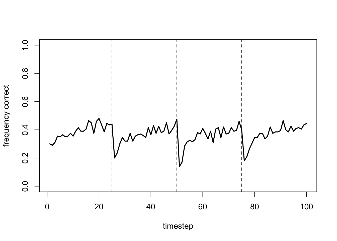
In each time period, the frequency of correct arm choices increases from chance (25%) to around 40%. While not amazing, some agents at least are successfully learning the optimal arm. And they are doing this despite environmental change and noisy rewards.
We now add heterogeneity via \(\alpha_\sigma\) and \(\beta_\sigma\):
data_model17b <- RL_multiple(N = 200,
                             alpha_mu = 0.7,
                             alpha_sd = 0.1,
                             beta_mu = 0.3,
                             beta_sd = 0.1)

plot_correct(data_model17b)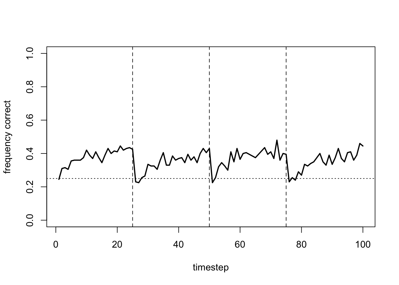
There is not too much difference here with just a small amount of random variation in the parameters. However, adding too much heterogeneity has a negative effect:
data_model17b <- RL_multiple(N = 200,
                             alpha_mu = 0.7,
                             alpha_sd = 1,
                             beta_mu = 0.3,
                             beta_sd = 1)

plot_correct(data_model17b)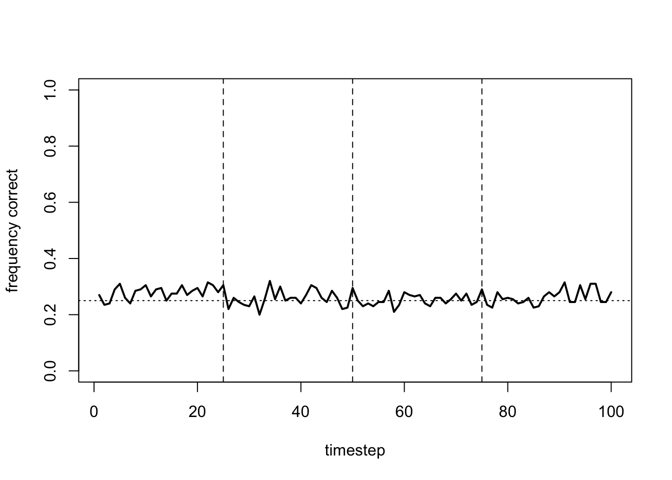
Now the proportion of optimal choices remain at chance. With too much heterogeneity we lose the exploration-exploitation balance that the values \(\alpha = 0.7\) and \(\beta = 0.3\) give us. Instead, most agents are either too exploitative or too exploratory and fail to learn.
To illustrate this further, we can remove heterogeneity and increase \(\beta_\mu\):
data_model17b <- RL_multiple(N = 200,
                             alpha_mu = 0.7,
                             alpha_sd = 0,
                             beta_mu = 5,
                             beta_sd = 0)

plot_correct(data_model17b)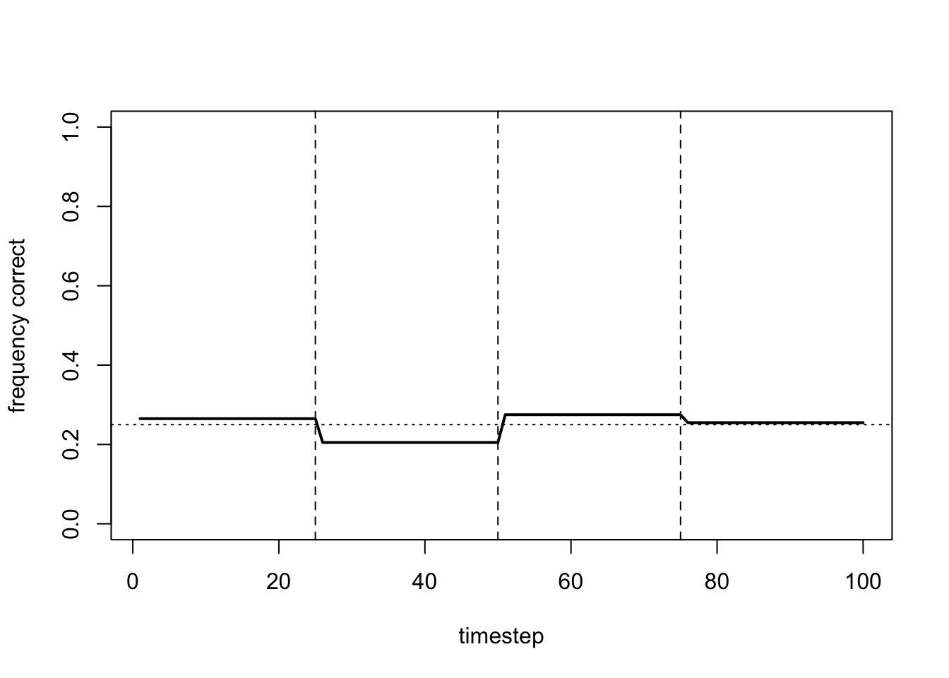
Now agents are too greedy, never exploring other arms and never learning the optimal arm. Indeed, the flat lines indicate that agents never switch arms at all.
Making \(\beta_\mu\) too low also eliminates learning, as agents are too exploratory and fail to exploit the optimal:
data_model17b <- RL_multiple(N = 200,
                             alpha_mu = 0.7,
                             alpha_sd = 0,
                             beta_mu = 0.1,
                             beta_sd = 0)

plot_correct(data_model17b)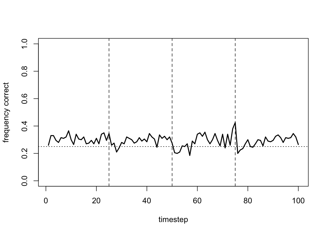
Rather than flat lines, this gives fluctuating lines as agents continually switch arms, never settling on the optimal.
Here then we have more robustly confirmed the results obtained with RL_single, demonstrating that this reinforcement learning algorithm with suitable values of \(\alpha\) and \(\beta\) leads on average to the learning of an optimal choice despite environmental change and noisy rewards.
Model 17c: Reinforcement learning plus social learning
Now that we have multiple agents all learning alongside each other, we can add social learning. Agents will be able to update their Q values not only using their own personal rewards, but also the choices of the other agents.
To implement social learning we use two new parameters, \(s\) and \(f\). \(s\) is defined as the probability on each trial that an agent engages in social learning, rather than the reinforcement learning as modelled above. When \(s = 0\), social learning is never used, and we revert to Model 17b. As \(s\) increases, social learning is more likely.
If social learning is used, it takes the form of unbiased cultural transmission (see Model 1) or conformist cultural transmission (see Model 5). Unlike in Model 5, we use a slightly different way of implementing conformist transmission. This way is less intuitive to understand, but easier to implement in this context.
We assume that the probability that an agent chooses arm \(i\), \(p_i\), is given by:
\[ p_i = \frac{n_i^f}{\sum_{j=1} ^k {n_j^f}} \hspace{30 mm}(17.2)\]
where \(n_i\) is the number of agents in the population who chose arm \(i\) on the previous trial and \(f\) is a conformity parameter. This \(f\) parameter is technically different to the \(D\) used in Model 5, but has the same effect of controlling the strength of conformity. The denominator is the sum of \(n^f\) for all arms from 1 to \(k\), where in our case \(k = 4\).
When \(f = 1\), transmission is unbiased. Anything to the power of 1 is unchanged, so the equation above simply gives the frequency of arm \(i\) in the population. When \(f > 1\), there is conformity in the sense defined in Model 5, i.e. more popular arms are disproportionately more likely to be chosen relative to unbiased transmission. To see this, here is a plot for two arms (\(k = 2\)), comparable to the two traits we simulated in Model 5, with \(N = 100\) and \(f = 2\):
N <- 100  # number of agents
f <- 2 # conformity strength
n <- 1:N  # number of N agents who picked arm 1; arm 2 is then N-n
freq <- n / N  # frequencies of arm 1
prob <- n^f / (n^f + (N-n)^f)  # probabilities according to equation above

plot(freq,
     prob,
     type = 'l',
     xlab = "frequency of arm 1",
     ylab = "probability of choosing arm 1")

abline(a = 0, b = 1, lty = 3)  # dotted line for unbiased transmission baseline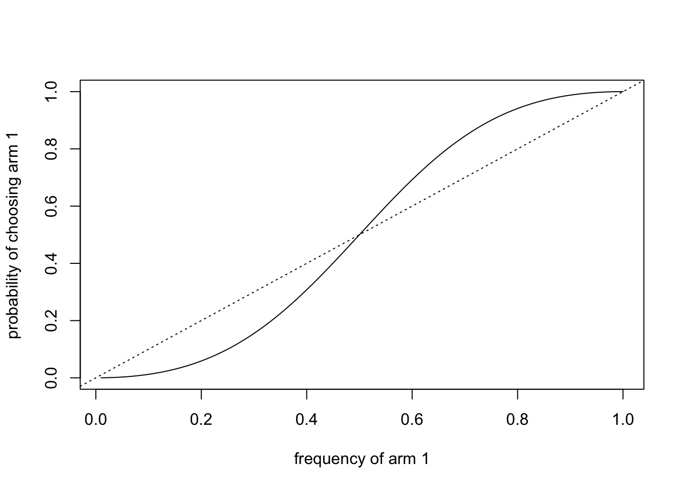
Here we see the familiar S-shaped conformity curve from Model 5. When a majority of agents pick arm 1 (frequency > 0.5), there is a greater than expected probability of picking arm 1 relative to unbiased transmission. When arm 1 is in the minority (frequency < 0.5), there is a less than expected probability. Just like \(D\), \(f\) acts to magnify the adoption of more-common traits. However, this formulation with \(f\) allows multiple traits - here, multiple arms - whereas the \(D\) formulation only permits two options.
Let’s start by assuming that all agents have identical \(s\) and \(f\) values, with \(\alpha\) and \(\beta\) still potentially varying across agents. The function RL_social below is largely identical to RL_multiple. However, instead of probs being the softmax probabilities derived from Q values, we instead store these softmax probabilities in a new variable p_RL (probabilities for reinforcement learning). On trial 1 (\(t == 1\)), probs is just p_RL, because there haven’t been any choices yet to use for social learning. On subsequent trials (\(t > 1\)), we also calculate p_SL (probabilities for social learning). First we get \(n[arm]\), the number of agents who chose each arm on trial \(t-1\). Then we apply our equation above to get p_SL. After converting p_SL into a matrix to make it comparable with p_RL, we combine p_RL and p_SL according to \(s\) to get overall probs. The rest is the same as before.
RL_social <- function(N, alpha_mu, alpha_sd, beta_mu, beta_sd, s, f) {

  # set up arm rewards
  arm_means <- data.frame(p1 = c(10,13,10,10),
                          p2 = c(10,10,10,13),
                          p3 = c(13,10,10,10),
                          p4 = c(10,10,13,10))
  arm_sd <- 1.5

  # draw agent beta, alpha, s and f from overall mean and sd
  beta <- rnorm(N, beta_mu, beta_sd)  # inverse temperatures
  alpha <- rnorm(N, alpha_mu, alpha_sd)  # learning rates

  # avoid impossible values
  alpha[alpha < 0] <- 0  # ensure all alphas are >0
  alpha[alpha > 1] <- 1  # ensure all alphas are <1
  beta[beta < 0] <- 0  # ensure all betas are >0

  # for storing Q values for 4 arms on current trial, initially all zero
  Q_values <- matrix(data = 0,
                     nrow = N,
                     ncol = 4)

  # for storing choices and rewards per agent per trial
  output <- data.frame(trial = rep(1:100, each = N),
                       agent = rep(1:N, 100),
                       choice = rep(NA, 100*N),
                       reward = rep(NA, 100*N))

  # vector to hold frequencies of choices for conformity
  n <- rep(NA, 4)

  # t-loop
  for (t in 1:100) {

    # get asocial softmax probabilities p_RL from Q_values
    p_RL <- exp(beta * Q_values) / rowSums(exp(beta * Q_values))

    # get social learning probabilities p_SL from t=2 onwards
    if (t == 1) {

      probs <- p_RL

    } else {

      # get number of agents who chose each option
      for (arm in 1:4) n[arm] <- sum(output[output$trial == (t-1),]$choice == arm)

      # conformity according to f
      p_SL <- n^f / sum(n^f)

      # convert p_SL to N-row matrix to match p_RL
      p_SL <- matrix(p_SL, nrow = N, ncol = 4, byrow = T)

      # update probs by combining p_RL and p_SL according to s
      probs <- (1-s)*p_RL + s*p_SL

    }

    # choose an arm based on probs
    choice <- apply(probs, 1, function(x) sample(1:4, 1, prob = x))

    # get reward
    if (t <= 25) reward <- round(rnorm(N, mean = arm_means$p1[choice], sd = arm_sd))
    if (t > 25 & t <= 50) reward <- round(rnorm(N, mean = arm_means$p2[choice], sd = arm_sd))
    if (t > 50 & t <= 75) reward <- round(rnorm(N, mean = arm_means$p3[choice], sd = arm_sd))
    if (t > 75) reward <- round(rnorm(N, mean = arm_means$p4[choice], sd = arm_sd))

    # update Q values one arm at a time
    for (arm in 1:4) {

      chosen <- which(choice==arm)

      Q_values[chosen,arm] <- Q_values[chosen,arm] +
        alpha[chosen] * (reward[chosen] - Q_values[chosen,arm])

    }

    # store choice and reward in output
    output[output$trial == t,]$choice <- choice
    output[output$trial == t,]$reward <- reward

  }

  # record whether correct
  output$correct <- output$choice == c(rep(2,25*N),rep(4,25*N),rep(1,25*N),rep(3,25*N))

  # export output dataframe
  output

}
If we set \(s = 0\) - no social learning - we should recapitulate RL_multiple. Note that when \(s = 0\), \(f\) is irrelevant as conformity cannot occur when there is no social learning.
data_model17c <- RL_social(N = 200,
                          alpha_mu = 0.7,
                          alpha_sd = 0.1,
                          beta_mu = 0.3,
                          beta_sd = 0.1,
                          s = 0,
                          f = 1)

plot_correct(data_model17c)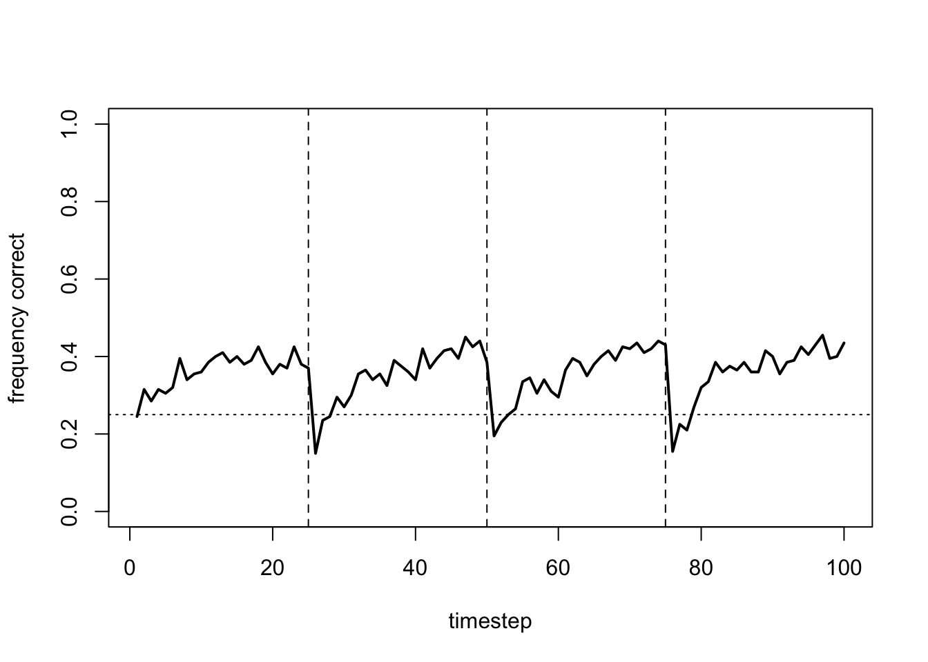
As before, the frequency of optimal arm choices increases in each time period to around 40%.
What happens if we add some social learning, \(s = 0.3\)?
data_model17c <- RL_social(N = 200,
                          alpha_mu = 0.7,
                          alpha_sd = 0.1,
                          beta_mu = 0.3,
                          beta_sd = 0.1,
                          s = 0.3,
                          f = 1)

plot_correct(data_model17c)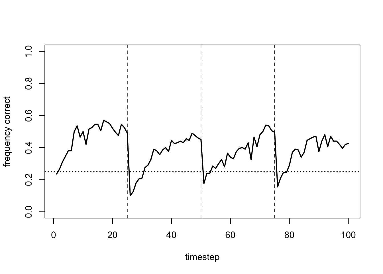
Adding some social learning improves the performance of our agents slightly. The proportion of correct choices now exceeds 40% by the end of most time periods. Social learning is magnifying the effect of reinforcement learning. Those agents who are engaging in reinforcement learning are on average learning and choosing the optimal arm, and agents who are engaging in social learning are therefore more likely to copy this more-frequent arm than the other less-frequent arms.
What about conformity, say \(f = 2\)?
data_model17c <- RL_social(N = 200,
                          alpha_mu = 0.7,
                          alpha_sd = 0.1,
                          beta_mu = 0.3,
                          beta_sd = 0.1,
                          s = 0.3,
                          f = 2)

plot_correct(data_model17c)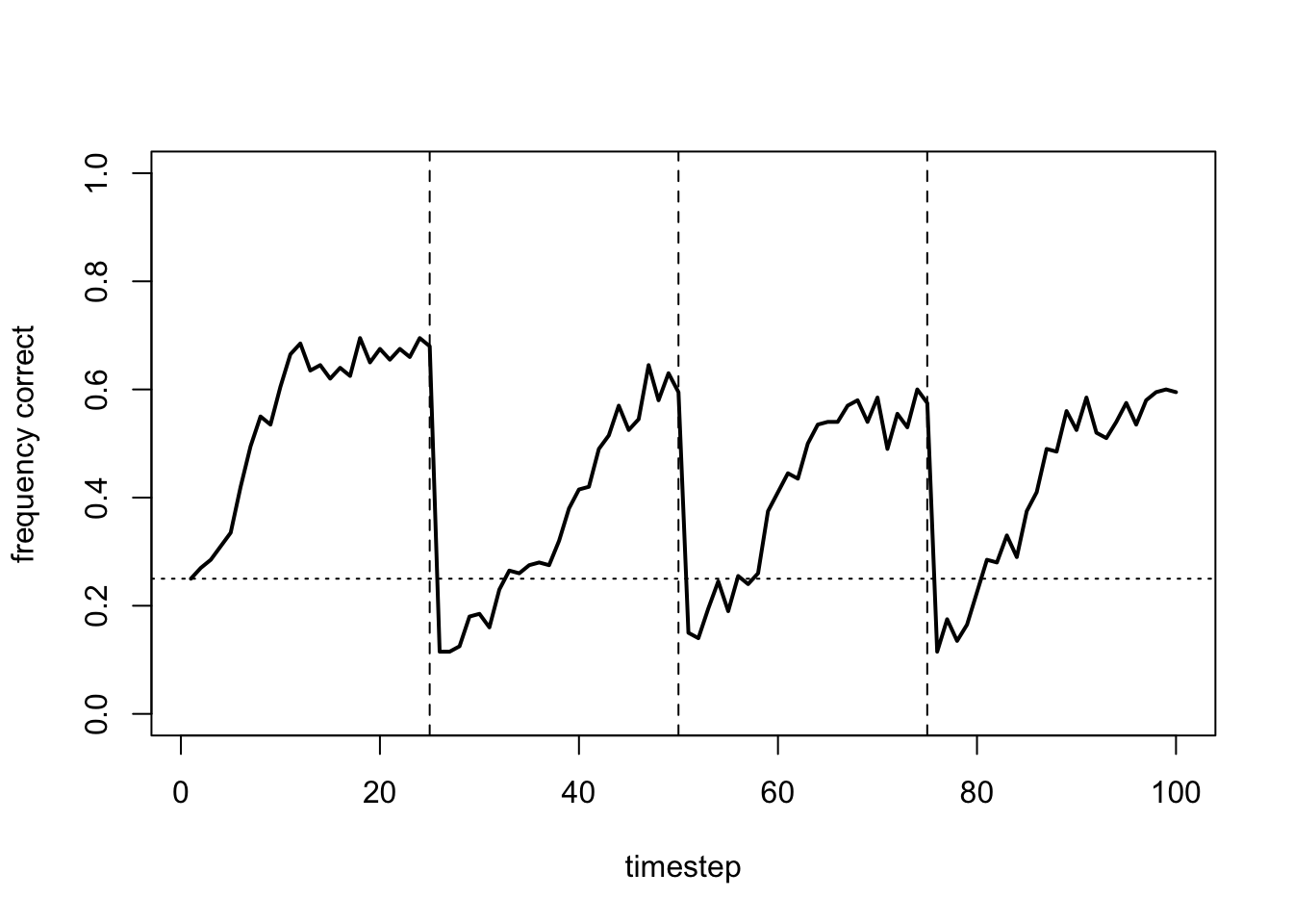
This is even better, with 60-70% of agents now making optimal choices by the end of each time period. Conformity magnifies reinforcement learning even more than unbiased social learning, given that reinforcement learning makes the optimal arm the most-common arm and conformity disproportionately increases this arm’s frequency.
However, too much social learning is not good. Here we increase \(s\) to 0.8:
data_model17c <- RL_social(N = 200,
                          alpha_mu = 0.7,
                          alpha_sd = 0.1,
                          beta_mu = 0.3,
                          beta_sd = 0.1,
                          s = 0.8,
                          f = 2)

plot_correct(data_model17c)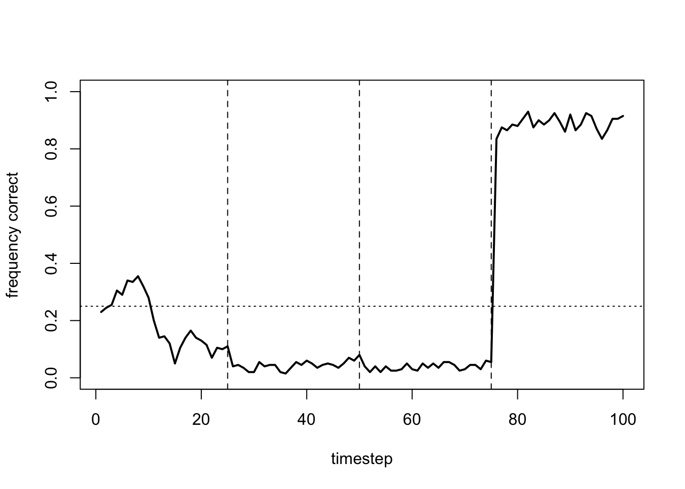
The output should show one time period at almost 100% correct choices, and the other three at almost 0%. With too much social learning, agents mostly make choices based on what others are choosing. Too few agents are using reinforcement / individual learning to discover the optimal arm. Instead, one arm goes to fixation due to cultural drift. In one time period it happens to be optimal, in the others it isn’t, and which one is purely due to chance.
Finally, we can add agent heterogeneity in both \(s\) and \(f\), just as we did for \(\alpha\) and \(\beta\). It seems reasonable that real people vary in both their propensity to copy others and their propensity for conformity, so we should be able to simulate these individual differences.
The following updated RL_social function draws \(s\) and \(f\) from normal distributions with means \(s_\mu\) and \(f_\mu\) and standard deviations \(s_\sigma\) and \(f_\sigma\) respectively. Note the new conformity code, which creates a matrix of \(n\) for each agent, raises it to the power of that agent’s \(f\) value, and divides by the sum of all the \(n^f\) values. This is a bit opaque, but as before this vectorised code is much faster than looping through all agents.
RL_social <- function(N,
                      alpha_mu, alpha_sd,
                      beta_mu, beta_sd,
                      s_mu, s_sd,
                      f_mu, f_sd) {

  # set up arm rewards
  arm_means <- data.frame(p1 = c(10,10,10,13),
                          p2 = c(10,13,10,10),
                          p3 = c(13,10,10,10),
                          p4 = c(10,10,13,10))
  arm_sd <- 1.5

  # draw agent beta, alpha, s and f from overall mean and sd
  beta <- rnorm(N, beta_mu, beta_sd)  # inverse temperatures
  alpha <- rnorm(N, alpha_mu, alpha_sd)  # learning rates
  s <- rnorm(N, s_mu, s_sd)  # social learning tendency
  f <- rnorm(N, f_mu, f_sd)  # conformity parameter

  # avoid impossible values
  alpha[alpha < 0] <- 0  # ensure all alphas are >0
  alpha[alpha > 1] <- 1  # ensure all alphas are <1
  beta[beta < 0] <- 0  # ensure all betas are >0
  s[s < 0] <- 0  # s between 0 and 1
  s[s > 1] <- 1
  f[f < 0] <- 0  # f > 0

  # for storing Q values for 4 arms on current trial, initially all zero
  Q_values <- matrix(data = 0,
                     nrow = N,
                     ncol = 4)

  # for storing choices and rewards per agent per trial
  output <- data.frame(trial = rep(1:100, each = N),
                       agent = rep(1:N, 100),
                       choice = rep(NA, 100*N),
                       reward = rep(NA, 100*N))

  # vector to hold frequencies of choices for conformity
  n <- rep(NA, 4)

  # t-loop
  for (t in 1:100) {

    # get asocial softmax probabilities p_RL from Q_values
    p_RL <- exp(beta * Q_values) / rowSums(exp(beta * Q_values))

    # get social learning probabilities p_SL from t=2 onwards
    if (t == 1) {

      probs <- p_RL

    } else {

      # get number of agents who chose each option
      for (arm in 1:4) n[arm] <- sum(output[output$trial == (t-1),]$choice == arm)

      # conformity according to f, allowing for different agent f's if f_sd>0
      p_SL <- matrix(rep(n, times = N)^rep(f, each = 4), nrow = N, ncol = 4, byrow = T)
      p_SL_rowsums <- matrix(rep(rowSums(p_SL), each = 4), nrow = N, ncol = 4, byrow = T)
      p_SL <- p_SL / p_SL_rowsums

      # update probs by combining p_RL and p_SL according to s
      probs <- (1-s)*p_RL + s*p_SL

    }

    # choose an arm based on probs
    choice <- apply(probs, 1, function(x) sample(1:4, 1, prob = x))

    # get reward
    if (t <= 25) reward <- round(rnorm(N, mean = arm_means$p1[choice], sd = arm_sd))
    if (t > 25 & t <= 50) reward <- round(rnorm(N, mean = arm_means$p2[choice], sd = arm_sd))
    if (t > 50 & t <= 75) reward <- round(rnorm(N, mean = arm_means$p3[choice], sd = arm_sd))
    if (t > 75) reward <- round(rnorm(N, mean = arm_means$p4[choice], sd = arm_sd))

    # update Q values one arm at a time
    for (arm in 1:4) {

      chosen <- which(choice==arm)

      Q_values[chosen,arm] <- Q_values[chosen,arm] +
        alpha[chosen] * (reward[chosen] - Q_values[chosen,arm])

    }

    # store choice and reward in output
    output[output$trial == t,]$choice <- choice
    output[output$trial == t,]$reward <- reward

  }

  # record whether correct
  output$correct <- output$choice == c(rep(4,25*N),rep(2,25*N),rep(1,25*N),rep(3,25*N))

  # export output dataframe
  output

}
We can confirm that the last output above is recreated with agent heterogeneity in \(\alpha\), \(\beta\), \(s\) and \(f\):
data_model17c <- RL_social(N = 200,
                           alpha_mu = 0.7,
                           alpha_sd = 0.1,
                           beta_mu = 0.3,
                           beta_sd = 0.1,
                           s_mu = 0.3,
                           s_sd = 0.1,
                           f_mu = 2,
                           f_sd = 0.1)

plot_correct(data_model17c)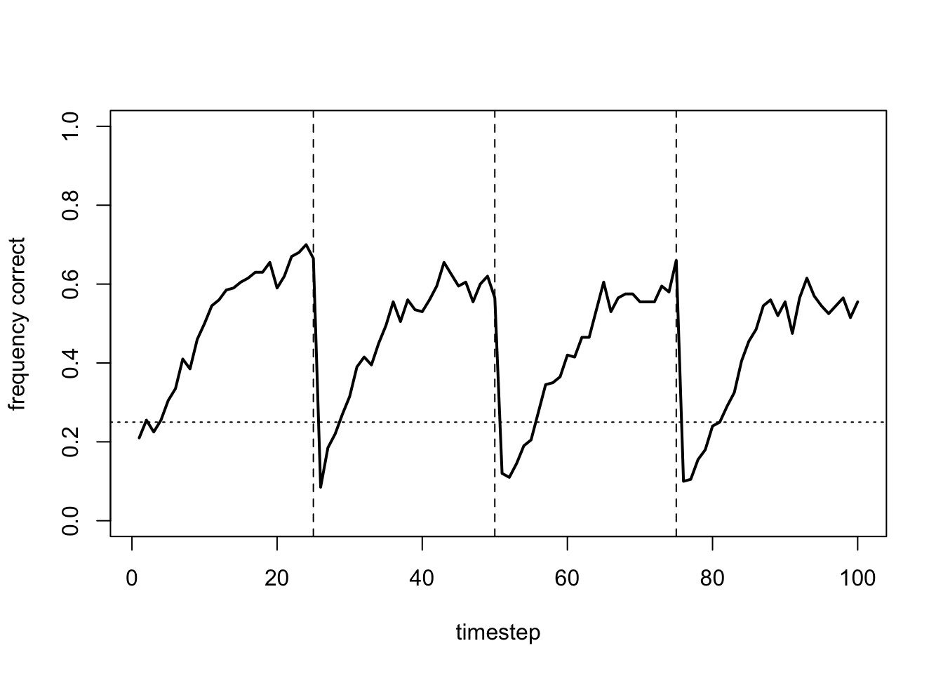
While it may seem trivial to show that adding a small amount of random variation to parameters gives the same output as not having any variation, it is useful in principle to be able to simulate agent heterogeneity in model parameters. In reality individual heterogeneity in learning and behaviour is the norm. In the Statistical Appendix below we will see how to recover these individually-varying parameters from our simulated data. This serves as a validation check for experiments and real-world data, where we might want to estimate these parameters from actual, individually-varying people.
Summary
In Model 17 we saw how to implement reinforcement learning. Cultural evolution models require some kind of individual learning to introduce variation and track environmental change. Reinforcement learning, extensively used in artificial intelligence and computer science, is a richer form of individual learning than something like cultural mutation seen in Model 2.
Our reinforcement learning algorithm is designed to balance exploitation and exploration in the multi-armed bandit task with hidden optima and noisy reward feedback. Too much exploitation means that the agent might prematurely settle on a non-optimal choice. Too much exploration and the agent will continue to try all options, never settling on the optimal choice. The parameters \(\alpha\) (the learning rate) and \(\beta\) (inverse temperature) can be used to balance this trade-off.
We also saw how social learning can magnify reinforcement learning, particularly conformist social learning. Conformity boosts the frequency of the most common option. If reinforcement learning has increased the frequency of the optimal option even slightly above chance, then conformity can boost the frequency of this optimal option further. However, too much social learning is bad. If there is not enough reinforcement learning going on, the optimal option is not discovered, and so a random arm is magnified.
Reinforcement learning has commonly been used in model-driven cultural evolution lab experiments such as McElreath et al. (2008), Barrett et al. (2017), Toyokawa et al. (2019) and Deffner et al. (2020). These experiments get participants to play a multi-armed bandit task of the kind simulated above. Rather than using generic statistical models such as linear regression to analyse the participant’s data, these studies use the reinforcement and social learning models implemented above. Participant data is fit to these models, and model parameters estimated both for the whole sample and for each participant. Some participants might be particularly exploratory, reflected in a low estimated \(\beta\). Some might be particularly prone to conformity, reflected in a large estimated \(f\). This is why we simulated agent heterogeneity - to reflect this real life heterogeneity. Overall, these experiments have shown that real participants are often quite effective at solving the multi-armed bandit task, both in balancing the exploitation-exploration trade-off and in using conformist social learning.
One might wonder about the ecological validity of multi-armed bandit tasks. Most of us rarely find ourselves faced with the task of choosing one of \(k\) slot machines in a casino. However, the general structure of the task probably resembles many real world problems beyond the windowless walls of a casino. For example, we might want to decide which of several restaurants have the best food; which beach has the fewest people; or which website gives the cheapest travel tickets. In each case, you do not know in advance which option is best; feedback is noisy (e.g. you might visit a restaurant on a day when they’ve run out of your favourite dish); and it’s possible to learn from others’ choices (e.g. by seeing how busy the restaurant is). The exploitation-exploration trade-off is inherent in all these real world examples of information search.
In terms of programming techniques, one major innovation is the introduction of agent heterogeneity in model parameters. Rather than assuming that every agent has the same, say, conformity parameter, we assume each agent differs. Formally, agent parameter values are drawn randomly from a normal distribution, with the standard deviation of this normal distribution controlling the amount of heterogeneity. However there is no reason that this has to be a normal distribution. Other distributions might better reflect real world individual variation.
We also saw a different way of modelling conformity to the one introduced in Model 5. While less intuitive than the ‘mating tables’ approach used to derive equation 5.1, equation 17.2 has the advantage of allowing any number of choices rather than just two. That makes it useful for the multi-armed bandit task when \(k > 2\).
Acknowledgements
The following resources were invaluable in compiling Model 17: Raphael Geddert’s Reinforcement Learning Resource Guide & Tutorial (https://github.com/rmgeddert/Reinforcement-Learning-Resource-Guide/blob/master/RLResourceGuide.md), Lei Zhang’s Bayesian Statistics and Hierarchical Bayesian Modeling for Psychological Science (https://github.com/lei-zhang/BayesCog_Wien) course, and Dominik Deffner’s analysis code for his 2020 study (https://github.com/DominikDeffner/Dynamic-Social-Learning). Many thanks also to Dominik Deffner who helped with the Stan code in the Statistical Appendix.
Exercises
Use RL_single to explore different values of \(\alpha\) and \(\beta\). Using code from previous models, write a function to generate a heatmap showing the proportion correct arm for a range of values of each parameter.
In Model 17 we started the agents with Q values all initially zero. As rewards are obtained, these Q values then increased. Try instead very high starting values, e.g. all 100. These will then decrease. Does this change the dynamics of RL_multiple shown in the plots? (see Sutton & Barto 2018 for discussion)
Use RL_social to explore different values of \(s\) and \(f\), using the heatmap function from (1) with fixed \(\alpha\) and \(\beta\). What happens when \(s = 1\)? What about when \(s = 0.3\) and \(f = 10\)? Explain these dynamics in terms of the findings regarding unbiased transmission in Model 1 and conformity in Model 5.
Modify the Model 17 functions to make the number of arms \(k\), the standard deviation of the arm reward distribution \(arm_sd\), and the number of timesteps \(t_{max}\), user-defined parameters. Instead of changing the optimal arm at fixed intervals, add another parameter which specifies the probability on each timestep of a new random arm becoming the optimal. Explore how the reinforcement learning algorithm handles different numbers of arms, different arm noisinesses, and different rates of environmental change.
Statistical Appendix
As discussed above, it is useful to be able to recover the model parameters (in our case \(\alpha\), \(\beta\), \(s\) and \(f\)) from the output simulation data. This serves as a validity check when running the same analyses on experimental or observational data generated by real people (or other animals), where we don’t know the parameter values.
Here we follow studies such as McElreath et al. (2008), Barrett et al. (2017), Toyokawa et al. (2019) and Deffner et al. (2020) and use multi-level Bayesian statistical models run using the platform Stan (https://mc-stan.org/). McElreath (2020) provides an excellent overview of Bayesian statistics in R and Stan. I won’t discuss the statistical methods used here but I recommend working through McElreath’s book to understand them fully.
We will use the cmdstanr package to interface with Stan. Follow the instructions to install cmdstanr at https://mc-stan.org/cmdstanr/articles/cmdstanr.html. You will also need to install CmdStan, the command line interface to Stan, and check you have a suitable C++ toolchain (don’t worry, you don’t need to understand what this is, just follow the instructions via the link). We will also use the bayesplot package to generate some plots later. This can be installed via CRAN like most other packages.
First we try to recover \(\alpha\) and \(\beta\) from a run of RL_single. We run the simulation and remind ourselves of the output:
##   arm1 arm2 arm3    arm4 choice reward correct
## 1    0    0  0.0  9.1000      4     13    TRUE
## 2    0    0  0.0 12.5300      4     14    TRUE
## 3    0    0  0.0 14.9590      4     16    TRUE
## 4    0    0  7.0 14.9590      3     10   FALSE
## 5    0    0  7.0 11.4877      4     10    TRUE
## 6    0    0 11.2 11.4877      3     13   FALSE
Our Stan model will only use choices and rewards from this output. These need to be in the form of a list rather than a dataframe, which we call dat:
## $choice
##   [1] 4 4 4 3 4 3 4 3 4 4 3 4 3 4 3 4 3 4 4 3 4 4 4 4 3 3 4 3 3 4 4 4 4 3 4 2 4
##  [38] 3 2 2 3 2 2 4 2 3 3 2 3 4 2 3 2 4 4 4 3 2 3 1 3 4 4 3 4 2 1 1 1 1 2 4 4 2
##  [75] 4 4 4 1 4 1 4 2 1 3 3 3 2 2 3 2 2 4 3 1 3 1 2 4 3 2
##
## $reward
##   [1] 13 14 16 10 10 13 12 10 14 13 11 10 10 13 12 14 14 14 13 11 15 11 15 12 14
##  [26] 10  9  8  8  9  9  8 12  7  9 12  7 10 17 12 11 13 15  8 12 11 10 17 12 10
##  [51] 11  7 11  7 11 11  9  8 10 13  9  9 10 10  8  9 13 13 15 12 11 12 10 10 11
##  [76]  9 11 11  9 11  9 12  9 15 15 14 10 12 10  9 10 10 10 12 12 10 10  8 17  8
Stan requires models written in the Stan programming language. This is slightly different to R. Usually the Stan model is saved as a separate text file with the extension .stan. This .stan file is then called within R to actually run the model. We will follow this practice. All the .stan files we will use are in the folder model17_stanfiles. The first one is called model17_single.stan. I will reproduce chunks of these stan files here but include eval=FALSE in the code chunks so that they are not run if you knit the RMarkdown file. If you are following along, don’t run these code chunks (you’ll just get an error).
Stan files require at least three sections. The first, labelled data, specifies the data that is required by the model. This should match the dat list from above. The data section of model17_single.stan is reproduced below:
Here we have our reward and choice variables. There are a few differences in this Stan code compared to R code. First, all statements must end in a semicolon. Second, comments are marked with // rather than #. Third, Stan requires the programmer to explicitly declare what type each variable is, i.e. whether it is an integer, real (continuous) number, vector, matrix or whatever (such languages are called ‘statically typed’, as opposed to R which is ‘dynamically typed’). The possible range of each variable can also be specified. The advantage of this explicit type declaration is that Stan throws an error if you try to do a calculation with, say, an integer when a real number is required, or mistakenly enter a value of 100 for a variable that is constrained to be between 1 and 10.
Hence choice and reward are both declared as arrays of 100 integers (int). An array is like a vector, but vectors in Stan must be real, while our variables are int, so we use arrays instead. choice is additionally constrained between 1 and 4 using the code <lower=1,upper=4> given that we only have four arms.
The second Stan block is parameters, where we declare the parameters of the model that we want Stan to estimate. For RL_single these are \(\alpha\) and \(\beta\):
parameters {
  real<lower = 0, upper = 1> alpha; // learning rate
  real<lower = 0> beta; // inverse temperature
}
Both our parameters are real, i.e. continuous. We constrain \(\alpha\) to be between 0 and 1, and \(\beta\) to be positive.
The final block in the Stan file is the model. This essentially recreates the simulation contained in RL_single, but instead of generating choices and rewards from probs and arm_means respectively, we use the already-generated choice and reward data in dat. We also omit output, because that’s already been generated.
model {
  vector[4] Q_values; // Q values for each arm
  vector[4] probs; // probabilities for each arm

  // priors
  alpha ~ beta(1,1);
  beta ~ normal(0,3);

  // initial Q values all zero
  Q_values = rep_vector(0,4);

  // trial loop
  for (t in 1:100) {

    // get softmax probabilities from Q_values
    probs = softmax(beta * Q_values);

    // choose an arm based on probs
    choice[t] ~ categorical(probs);

    //update Q_values
    Q_values[choice[t]] = Q_values[choice[t]] +
      alpha * (reward[t] - Q_values[choice[t]]);

  }

}
The first two lines above declare Q_values and probs as vectors (hence real numbers) of length four, one for each arm. We then specify priors for \(\alpha\) and \(\beta\). Recall from Model 16 that Bayesian analyses require a prior distribution, which is updated given data to generate a posterior distribution. Because \(\alpha\) must range from 0 to 1 and we don’t have strong expectations about what it might be (remember, we are assuming that we haven’t already seen the simulated output, just like we wouldn’t know what the experimental participants’ \(\alpha\)s are), we specify a flat beta distribution. Recall again from Model 16 that a beta distribution must range from 0 to 1, and with parameters (1,1) this gives a flat uniform distribution. For \(\beta\) we can expect that relatively low values are more likely; \(\beta\) has no upper bound, but something like 0.5 or 1 is more likely than 1000 or 10000. We therefore specify a normal distribution peaking at 0. Remember that \(\beta\) was constrained to be positive in the parameters section so the prior is cut at zero and can’t be negative.
Then like in RL_single we set initial Q_values to all be zero and start the t-loop. probs is calculated as in RL_single but using Stan’s built-in softmax function rather than explicitly writing out the softmax formula. The choice for this trial is then modelled using the categorical distribution, and Q_values are updated as before using the reward for this trial.
Now we have all three blocks of the Stan file we can load the model into R using the cmdstan_model command, specifying the Stan file location. At this point, any programming errors or inconsistencies in your Stan file might be flagged. We then sample the model using the sample command, specifying the data list dat, the number of chains and number of warmup and sampling iterations. Chains refers to the number of Markov chains, and iterations to the length of those chains. Warmup chains are not used to derive estimates of your parameters, which only come from the sampling iterations. See McElreath (2020) for an explanation of these terms. Essentially though, the more chains and the more iterations, the more robust will be the model estimates. On the other hand, the more chains and iterations, the longer the model will take to run. Good advice is to run several short chains to ensure that the chains converge well and the model is working properly, then one long chain for the final analysis. Here we will run 1 chain with 500 warmup and 500 sampling iterations. Try more chains and iterations to compare.
# load stan model from file
RL_single_stan <- cmdstan_model("model17_stanfiles/model17_single.stan")

# run model
fit_RL_single <- RL_single_stan$sample(
  data = dat,
  chains = 1,
  iter_warmup = 500,
  iter_sampling = 500)
## Running MCMC with 1 chain...
##
## Chain 1 Iteration: 1 / 1000 [ 0%] (Warmup)
## Chain 1 Iteration: 100 / 1000 [ 10%] (Warmup)
## Chain 1 Iteration: 200 / 1000 [ 20%] (Warmup)
## Chain 1 Iteration: 300 / 1000 [ 30%] (Warmup)
## Chain 1 Iteration: 400 / 1000 [ 40%] (Warmup)
## Chain 1 Iteration: 500 / 1000 [ 50%] (Warmup)
## Chain 1 Iteration: 501 / 1000 [ 50%] (Sampling)
## Chain 1 Iteration: 600 / 1000 [ 60%] (Sampling)
## Chain 1 Iteration: 700 / 1000 [ 70%] (Sampling)
## Chain 1 Iteration: 800 / 1000 [ 80%] (Sampling)
## Chain 1 Iteration: 900 / 1000 [ 90%] (Sampling)
## Chain 1 Iteration: 1000 / 1000 [100%] (Sampling)
## Chain 1 finished in 0.6 seconds.You will see a series of progress messages indicating the number of iterations completed and the time taken. To see the output, we use the print command with the Stan model and the parameters:
##  variable mean median   sd  mad   q5  q95 rhat ess_bulk ess_tail
##     alpha 0.79   0.81 0.12 0.14 0.59 0.97 1.03      134      121
##     beta  0.23   0.23 0.04 0.04 0.16 0.30 1.00      260      258
The key bits here are the estimated means of \(\alpha\) and \(\beta\) in the first column of the table. Hopefully our Stan model has estimated our parameters well and they are close to \(\alpha = 0.7\) and \(\beta = 0.3\). Given that there is only one agent and a relatively small number of timesteps, they are unlikely to be super accurate, and the 95% confidence intervals (q5 and q95) are probably quite wide.
The final columns of the table give a convergence diagnostic Rhat (\(\hat{R}\)) and two measures of the effective number of independent samples, ess_bulk and ess_tail. These are all indicators of how well the chains converged and how reliable the estimates are. See McElreath (2020) for discussion of these measures. In general, Rhat should be 1 and definitely no greater than 1.05, and ess_bulk and ess_tail should not be too low relative to the number of non-warmup iterations, which here was 500. An Rhat larger than 1 and very low ess indicate poorly converged chains and probably a misspecified model.
We can show the shape of the posterior distribution of each parameter using the mcmc_dens command from the bayesplot package:
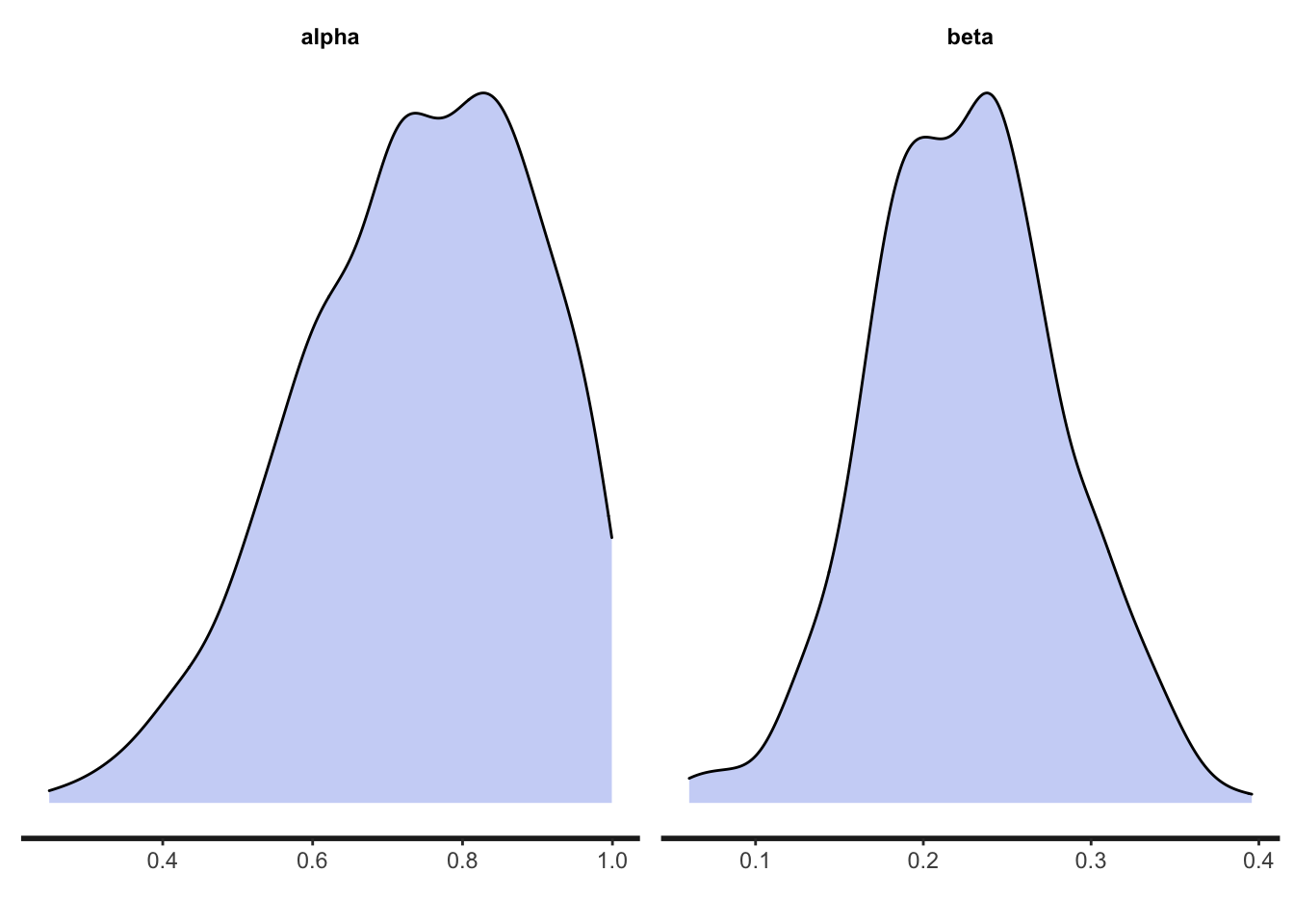
Hopefully the actual values of 0.7 and 0.3 fall within these posterior distributions.
Although our model converged well and produced reasonably accurate estimates, later models will be more complex and not converge so well. One way to deal with this is to convert the parameters to log and logit scales. We will do this here so that later on it doesn’t get confusing.
Converting parameters to log and logit scales is a way of constraining them to be positive and between 0 and 1 respectively. This is done in the Stan file model17_single_log.stan. In this file the parameters block of the Stan file is changed to:
Rather than \(\alpha\) and \(\beta\), our parameters to estimate are logit_alpha and log_beta. These are declared as unconstrained real (continuous) numbers. Then in the model block we define the priors for these as normal distributions, declare \(\alpha\) and \(\beta\) in the t-loop, and calculate them using inv_logit and exp on logit_alpha and log_beta respectively. Otherwise, everything is identical to before.
model {
  vector[4] Q_values; // Q values for each arm
  vector[4] probs; // probabilities for each arm

  // priors
  logit_alpha ~ normal(0,1);
  log_beta ~ normal(-1,1);

  // initial Q values all zero
  Q_values = rep_vector(0,4);

  // trial loop
  for (t in 1:100) {

    real alpha;
    real beta;

    // get softmax probabilities from Q_values
    beta = exp(log_beta);
    probs = softmax(beta * Q_values);

    // choose an arm based on probs
    choice[t] ~ categorical(probs);

    //update Q_values
    alpha = inv_logit(logit_alpha);
    Q_values[choice[t]] = Q_values[choice[t]] +
      alpha * (reward[t] - Q_values[choice[t]]);

  }

}
Finally, we add a new block called generated quantities to convert logit_alpha and log_beta back to \(\alpha\) and \(\beta\), rather than having to do this by hand afterwards:
generated quantities {
  real alpha;
  real beta;

  alpha = inv_logit(logit_alpha);
  beta = exp(log_beta);
}
Now we run our new model:
# load stan model from file
RL_single_log_stan <- cmdstan_model("model17_stanfiles/model17_single_log.stan")

# run model
fit_RL_single_log <- RL_single_log_stan$sample(
  data = dat,
  chains = 1,
  iter_warmup = 500,
  iter_sampling = 500)
## Running MCMC with 1 chain...
##
## Chain 1 Iteration: 1 / 1000 [ 0%] (Warmup)
## Chain 1 Iteration: 100 / 1000 [ 10%] (Warmup)
## Chain 1 Iteration: 200 / 1000 [ 20%] (Warmup)
## Chain 1 Iteration: 300 / 1000 [ 30%] (Warmup)
## Chain 1 Iteration: 400 / 1000 [ 40%] (Warmup)
## Chain 1 Iteration: 500 / 1000 [ 50%] (Warmup)
## Chain 1 Iteration: 501 / 1000 [ 50%] (Sampling)
## Chain 1 Iteration: 600 / 1000 [ 60%] (Sampling)
## Chain 1 Iteration: 700 / 1000 [ 70%] (Sampling)
## Chain 1 Iteration: 800 / 1000 [ 80%] (Sampling)
## Chain 1 Iteration: 900 / 1000 [ 90%] (Sampling)
## Chain 1 Iteration: 1000 / 1000 [100%] (Sampling)
## Chain 1 finished in 0.6 seconds.Again we use print to get the parameter estimates, specifying only \(\alpha\) and \(\beta\) rather than logit_alpha and log_beta:
##  variable mean median   sd  mad   q5  q95 rhat ess_bulk ess_tail
##     alpha 0.73   0.74 0.11 0.11 0.54 0.89 1.01      320      168
##     beta  0.23   0.22 0.04 0.04 0.16 0.30 1.00      415      281
They should be a good match with the estimates from fit_RL_single.
Next we do the same for RL_multiple, with individual heterogeneity in \(\alpha\) and \(\beta\). The simulated data looks like this:
data_model17b <- RL_multiple(N = 50,
                             alpha_mu = 0.7,
                             alpha_sd = 0.1,
                             beta_mu = 0.3,
                             beta_sd = 0.1)

head(data_model17b)
## trial agent choice reward correct
## 1 1 1 2 9 FALSE
## 2 1 2 1 8 FALSE
## 3 1 3 4 15 TRUE
## 4 1 4 1 9 FALSE
## 5 1 5 4 13 TRUE
## 6 1 6 4 13 TRUEWe now have a trial column and an agent column given that there are \(N = 50\) agents. As before, we need to convert these into a list. Instead of choice and reward being 100-length vectors, now we convert them to 100 x \(N\) matrices with each row a timestep as before but with each column representing an agent. These matrices are stored in dat along with \(N\).
# convert choice and reward to matrices, ncol=N, nrow=t_max
choice_matrix <- matrix(data_model17b$choice, ncol = max(data_model17b$agent), byrow = T)
reward_matrix <- matrix(data_model17b$reward, ncol = max(data_model17b$agent), byrow = T)

# create data list
dat <- list(choice = choice_matrix,
            reward = reward_matrix,
            N = max(data_model17b$agent))
The Stan file model17_multiple.stan contains the stan code for this analysis. The data block imports the three elements of dat. \(N\) is an int (integer; we can’t have half an agent). reward and choice are 100 x \(N\) arrays of integers (we could use matrices, but in Stan they can only hold real numbers, so arrays are preferable).
data {
  int N;  // number of agents
  array[100, N] int reward; // reward
  array[100, N] int<lower=1,upper=4> choice; // arm choice
}
Next the parameters block, along with a new transformed parameters block. As before we have logit_alpha and log_beta. But now there are several other parameters: \(z_i\), \(\sigma_i\), \(\rho_i\) and \(v_i\). These are all used to implement heterogeneity across agents, sometimes called varying effects or random effects in this context. Consult McElreath (2020) for an explanation of these parameters. The key one is \(v_i\) which gives the individual-level variation in each parameter. Note that the [2] associated with these parameters refers to the number of parameters that have varying effects (\(\alpha\) and \(\beta\)).
parameters {
  real logit_alpha; // learning rate grand mean
  real log_beta; // inverse temperature grand mean

  matrix[2, N] z_i;  // matrix of uncorrelated z-values
  vector<lower=0>[2] sigma_i; // sd of parameters across individuals
  cholesky_factor_corr[2] Rho_i; // cholesky factor
}

transformed parameters{
  matrix[2, N] v_i; // matrix of varying effects for each individual
  v_i = (diag_pre_multiply(sigma_i, Rho_i ) * z_i);
}
Finally we have the model block. There are a few changes to the previous single agent model. Q_values is now an \(N\) x 4 array in order to keep track of Q values for all \(N\) agents. There are priors for the new varying effects parameters, which again I leave you to consult McElreath (2020) for further explanation. Suffice to say that these are relatively flat priors with no strong expectations about the extent of the heterogeneity. Then we need to set up an \(i\)-loop to cycle through each agent within the \(t\)-loop. Vectorisation in Stan is possible but tricky, so I’ve kept it simple with an agent loop. The final change is that when calculating \(\alpha\) and \(\beta\) for each agent, we add that agent’s \(v_i\) term. This is indicated by the first index of \(v_i\), so \(v_i\)[1,i] gives the varying effect for \(\alpha\) for agent i and \(v_i\)[2,i] gives the varying effect for \(\beta\) for agent i. The rest is the same as before.
model {
  array[N] vector[4] Q_values; // Q values per agent
  vector[4] probs; // probabilities for each arm

  // priors
  logit_alpha ~ normal(0,1);
  log_beta ~ normal(-1,1);

  to_vector(z_i) ~ normal(0,1);
  sigma_i ~ exponential(1);
  Rho_i ~ lkj_corr_cholesky(4);

  // initial Q values all zero
  for (i in 1:N) Q_values[i] = rep_vector(0,4);

  // trial loop
  for (t in 1:100) {

    // agent loop
    for (i in 1:N) {

      real alpha;  // v_i parameter 1
      real beta;  // v_i parameter 2

      // get softmax probabilities from Q_values
      beta = exp(log_beta + v_i[2,i]);
      probs = softmax(beta * Q_values[i]);

      // choose an arm based on probs
      choice[t,i] ~ categorical(probs);

      //update Q_values
      alpha = inv_logit(logit_alpha + v_i[1,i]);
      Q_values[i,choice[t,i]] = Q_values[i,choice[t,i]] +
        alpha * (reward[t,i] - Q_values[i,choice[t,i]]);

    }

  }

}
The generated quantities block is identical to before.
generated quantities {
  real alpha;
  real beta;

  alpha = inv_logit(logit_alpha);
  beta = exp(log_beta);
}
Now we run the model:
# load stan model from file
fit_RL_multiple_stan <- cmdstan_model("model17_stanfiles/model17_multiple.stan")

# run model
fit_RL_multiple <- fit_RL_multiple_stan$sample(
  data = dat,
  chains = 1,
  iter_warmup = 500,
  iter_sampling = 500)
## Running MCMC with 1 chain...## Chain 1 Informational Message: The current Metropolis proposal is about to be rejected because of the following issue:## Chain 1 Exception: lkj_corr_cholesky_lpdf: Random variable[2] is 0, but must be positive! (in '/var/folders/qv/y7f3gq251kv68y9zxnr6cpbh0000gn/T/Rtmptonbtt/model-a05445f7bafc.stan', line 32, column 2 to column 31)## Chain 1 If this warning occurs sporadically, such as for highly constrained variable types like covariance matrices, then the sampler is fine,## Chain 1 but if this warning occurs often then your model may be either severely ill-conditioned or misspecified.## Chain 1## Chain 1 Informational Message: The current Metropolis proposal is about to be rejected because of the following issue:## Chain 1 Exception: lkj_corr_cholesky_lpdf: Random variable[2] is 0, but must be positive! (in '/var/folders/qv/y7f3gq251kv68y9zxnr6cpbh0000gn/T/Rtmptonbtt/model-a05445f7bafc.stan', line 32, column 2 to column 31)## Chain 1 If this warning occurs sporadically, such as for highly constrained variable types like covariance matrices, then the sampler is fine,## Chain 1 but if this warning occurs often then your model may be either severely ill-conditioned or misspecified.## Chain 1## Chain 1 Informational Message: The current Metropolis proposal is about to be rejected because of the following issue:## Chain 1 Exception: lkj_corr_cholesky_lpdf: Random variable[2] is 0, but must be positive! (in '/var/folders/qv/y7f3gq251kv68y9zxnr6cpbh0000gn/T/Rtmptonbtt/model-a05445f7bafc.stan', line 32, column 2 to column 31)## Chain 1 If this warning occurs sporadically, such as for highly constrained variable types like covariance matrices, then the sampler is fine,## Chain 1 but if this warning occurs often then your model may be either severely ill-conditioned or misspecified.## Chain 1## Chain 1 Iteration: 1 / 1000 [ 0%] (Warmup)## Chain 1 Informational Message: The current Metropolis proposal is about to be rejected because of the following issue:## Chain 1 Exception: lkj_corr_cholesky_lpdf: Random variable[2] is 0, but must be positive! (in '/var/folders/qv/y7f3gq251kv68y9zxnr6cpbh0000gn/T/Rtmptonbtt/model-a05445f7bafc.stan', line 32, column 2 to column 31)## Chain 1 If this warning occurs sporadically, such as for highly constrained variable types like covariance matrices, then the sampler is fine,## Chain 1 but if this warning occurs often then your model may be either severely ill-conditioned or misspecified.## Chain 1## Chain 1 Informational Message: The current Metropolis proposal is about to be rejected because of the following issue:## Chain 1 Exception: lkj_corr_cholesky_lpdf: Random variable[2] is 0, but must be positive! (in '/var/folders/qv/y7f3gq251kv68y9zxnr6cpbh0000gn/T/Rtmptonbtt/model-a05445f7bafc.stan', line 32, column 2 to column 31)## Chain 1 If this warning occurs sporadically, such as for highly constrained variable types like covariance matrices, then the sampler is fine,## Chain 1 but if this warning occurs often then your model may be either severely ill-conditioned or misspecified.## Chain 1## Chain 1 Iteration: 100 / 1000 [ 10%] (Warmup)
## Chain 1 Iteration: 200 / 1000 [ 20%] (Warmup)
## Chain 1 Iteration: 300 / 1000 [ 30%] (Warmup)
## Chain 1 Iteration: 400 / 1000 [ 40%] (Warmup)
## Chain 1 Iteration: 500 / 1000 [ 50%] (Warmup)
## Chain 1 Iteration: 501 / 1000 [ 50%] (Sampling)
## Chain 1 Iteration: 600 / 1000 [ 60%] (Sampling)
## Chain 1 Iteration: 700 / 1000 [ 70%] (Sampling)
## Chain 1 Iteration: 800 / 1000 [ 80%] (Sampling)
## Chain 1 Iteration: 900 / 1000 [ 90%] (Sampling)
## Chain 1 Iteration: 1000 / 1000 [100%] (Sampling)
## Chain 1 finished in 229.6 seconds.Here are the results:
## variable mean median sd mad q5 q95 rhat ess_bulk ess_tail
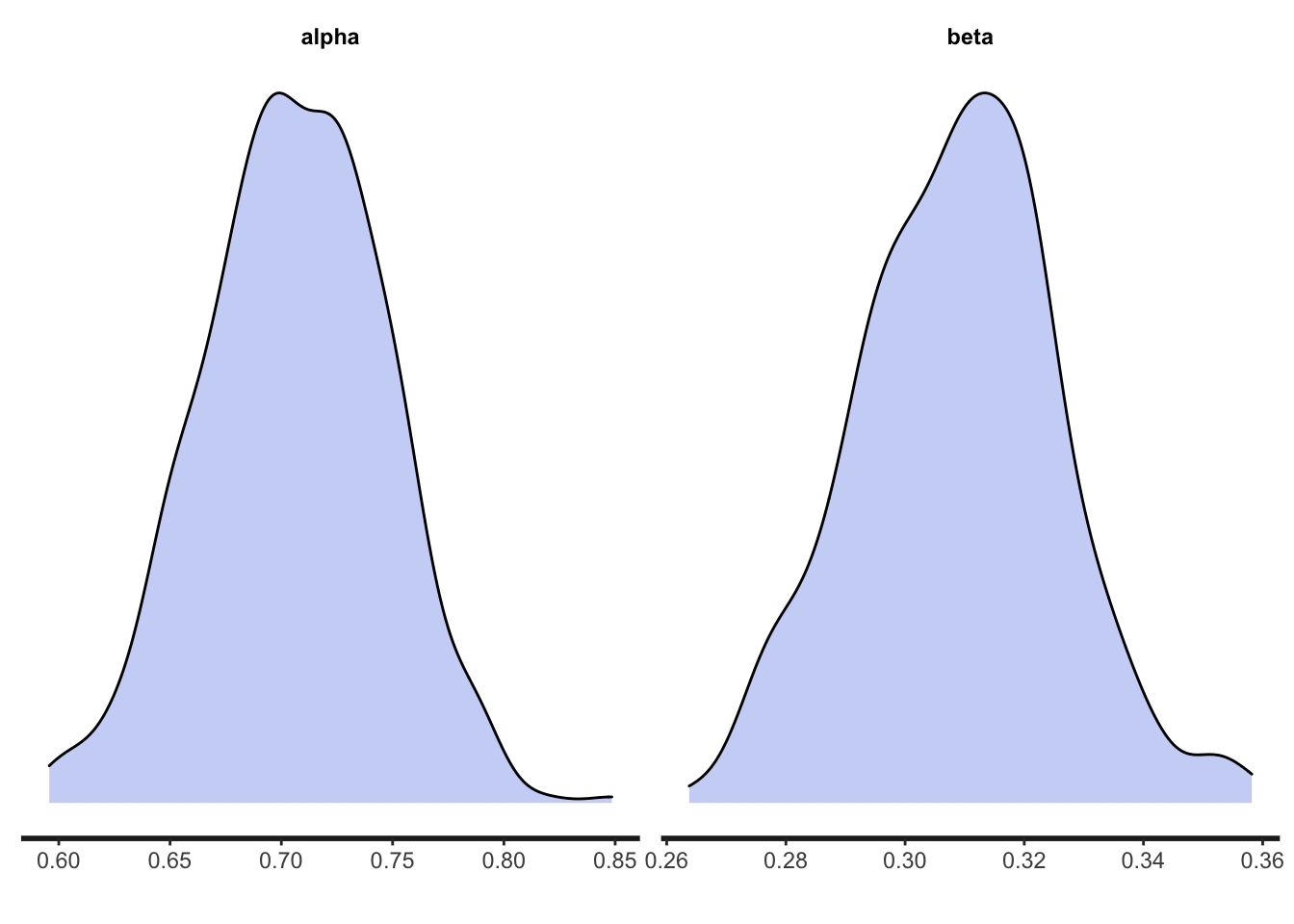
## alpha 0.70 0.70 0.03 0.03 0.65 0.75 1.00 353 397
## beta 0.30 0.30 0.02 0.02 0.27 0.33 1.00 307 219Hopefully the model accurately estimated the original parameter values of 0.7 and 0.3. Indeed, given that we now have much more data (5000 data points from \(N = 50\) rather than 100 data points from \(N = 1\)), these estimates should be more accurate than they were for RL_single as indicated by narrower confidence intervals. We can see the posteriors as before, which should also be more concentrated around the actual values:
And finally we run the whole analysis for RL_social:
data_model17c <- RL_social(N = 50,
                           alpha_mu = 0.7,
                           alpha_sd = 0.1,
                           beta_mu = 0.3,
                           beta_sd = 0.1,
                           s_mu = 0.3,
                           s_sd = 0.1,
                           f_mu = 2,
                           f_sd = 0.1)

head(data_model17c)
## trial agent choice reward correct
## 1 1 1 1 7 FALSE
## 2 1 2 2 7 FALSE
## 3 1 3 2 11 FALSE
## 4 1 4 3 9 FALSE
## 5 1 5 1 9 FALSE
## 6 1 6 2 13 FALSEThe output for RL_social is the same as for RL_multiple. As such the dat list is largely similar. However, to model conformity, we need for each timestep the number of agents on the previous timestep who chose each arm. The following code calculates the number of agents on each timestep who chose each arm and stores it in n_matrix, a 100 x 4 matrix with timesteps along the rows and arms along the columns.
# convert choice and reward to matrices, ncol=N, nrow=t_max
choice_matrix <- matrix(data_model17c$choice, ncol = max(data_model17c$agent), byrow = T)
reward_matrix <- matrix(data_model17c$reward, ncol = max(data_model17c$agent), byrow = T)

# create frequency matrix for conformity function
n_matrix <- matrix(nrow = 100, ncol = 4)
for (arm in 1:4) {
  for (t in 1:100) {
    n_matrix[t,arm] <- sum(data_model17c[data_model17c$trial == t,]$choice == arm)
  }
}

# create data list
dat <- list(choice = choice_matrix,
            reward = reward_matrix,
            N = max(data_model17c$agent),
            n = n_matrix)
Now we build our Stan file as before, which is saved as model17_social.stan. First, the data block contains \(N\), choices, rewards and the new n_matrix set of demonstrator numbers, entered as simply \(n\):
data {
  int N;  // number of agents
  array[100, N] int reward; // reward
  array[100, N] int<lower=1,upper=4> choice; // arm choice
  array[100, 4] int<lower=0,upper=N> n; // number of agents picking each arm
}
The parameters and transformed parameters now include the social learning parameter. The frequency of social learning, \(s\), is put on the logit scale as it is constrained to 0-1. The conformity parameter \(f\) is logged, as it is constrained to be positive. The varying effects parameters are now length 4 rather than 2, as there are now four parameters (\(\alpha\), \(\beta\), \(s\) and \(f\)).
parameters {
  real logit_alpha; // learning rate grand mean
  real log_beta; // inverse temperature grand mean
  real logit_s; // social learning prob grand mean
  real log_f; // conformity parameter grand mean

  matrix[4, N] z_i;  // matrix of uncorrelated z-values
  vector<lower=0>[4] sigma_i; // sd of parameters across individuals
  cholesky_factor_corr[4] Rho_i; // cholesky factor
}

transformed parameters{
  matrix[4,N] v_i; // matrix of varying effects for each individual
  v_i = (diag_pre_multiply(sigma_i, Rho_i ) * z_i);
}
And the model:
model {
  array[N] vector[4] Q_values; // Q values per agent
  vector[4] probs; // probabilities for each arm
  vector[4] p_RL; // reinforcement learning probabilities
  vector[4] p_SL; // social learning probabilities

  // priors
  logit_alpha ~ normal(0,1);
  log_beta ~ normal(-1,1);
  logit_s ~ normal(0,1);
  log_f ~ normal(-1,1);

  to_vector(z_i) ~ normal(0,1);
  sigma_i ~ exponential(1);
  Rho_i ~ lkj_corr_cholesky(4);

  // initial Q values all zero
  for ( i in 1:N ) Q_values[i] = rep_vector(0,4);

  // trial loop
  for (t in 1:100) {

    // agent loop
    for (i in 1:N) {

      real alpha;  // v_i parameter 1
      real beta;  // v_i parameter 2
      real s;  // v_i parameter 3
      real f;  // v_i parameter 4

      // get asocial softmax probabilities from Q_values
      beta = exp(log_beta + v_i[2,i]);
      p_RL = softmax(beta * Q_values[i]);

      if (t == 1) {

        // first generation has no social information
        probs = p_RL;

      } else {

        // from t=2 onwards, do conformity according to f

        f = exp(log_f + v_i[4,i]);
        for (arm in 1:4) p_SL[arm] = n[t-1,arm]^f;
        p_SL = p_SL / sum(p_SL);

        //update probs by combining p_RL and p_SL according to s
        s = inv_logit(logit_s + v_i[3,i]);
        probs = (1-s) * p_RL + s * p_SL;

      }

      // choose an arm based on probs
      choice[t,i] ~ categorical(probs);

      //update Q values
      alpha = inv_logit(logit_alpha + v_i[1,i]);
      Q_values[i,choice[t,i]] = Q_values[i,choice[t,i]] +
        alpha * (reward[t,i] - Q_values[i,choice[t,i]]);

    }

  }

}
Just as in the simulation, we define p_RL and p_SL as the probabilities for reinforcement and social learning respectively. From the second timestep onwards, we implement social learning. \(f\) is created from log_f and \(v_i\)[4,i] and \(s\) is created from logit_s and \(v_i\)[3,i], like we do for \(\alpha\) and \(\beta\). Now that we are not vectorising, the conformity equation is more straightforward, with each arm’s frequency on timestep \(t-1\) raised to the power of \(f\) and divided by the sum of all four arms.
And finally, generated quantities now includes \(s\) and \(f\):
generated quantities {
  real alpha;
  real beta;
  real s;
  real f;

  alpha = inv_logit(logit_alpha);
  beta = exp(log_beta);
  s = inv_logit(logit_s);
  f = exp(log_f);
}
Let’s run the model.
# load stan model from file
fit_RL_social_stan <- cmdstan_model("model17_stanfiles/model17_social.stan")

# run model
fit_RL_social <- fit_RL_social_stan$sample(
  data = dat,
  chains = 1,
  iter_warmup = 500,
  iter_sampling = 500)
## Running MCMC with 1 chain...## Chain 1 Informational Message: The current Metropolis proposal is about to be rejected because of the following issue:## Chain 1 Exception: lkj_corr_cholesky_lpdf: Random variable[3] is 0, but must be positive! (in '/var/folders/qv/y7f3gq251kv68y9zxnr6cpbh0000gn/T/Rtmptonbtt/model-a05420a5be91.stan', line 39, column 2 to column 31)## Chain 1 If this warning occurs sporadically, such as for highly constrained variable types like covariance matrices, then the sampler is fine,## Chain 1 but if this warning occurs often then your model may be either severely ill-conditioned or misspecified.## Chain 1## Chain 1 Informational Message: The current Metropolis proposal is about to be rejected because of the following issue:## Chain 1 Exception: lkj_corr_cholesky_lpdf: Random variable[3] is 0, but must be positive! (in '/var/folders/qv/y7f3gq251kv68y9zxnr6cpbh0000gn/T/Rtmptonbtt/model-a05420a5be91.stan', line 39, column 2 to column 31)## Chain 1 If this warning occurs sporadically, such as for highly constrained variable types like covariance matrices, then the sampler is fine,## Chain 1 but if this warning occurs often then your model may be either severely ill-conditioned or misspecified.## Chain 1## Chain 1 Informational Message: The current Metropolis proposal is about to be rejected because of the following issue:## Chain 1 Exception: lkj_corr_cholesky_lpdf: Random variable[3] is 0, but must be positive! (in '/var/folders/qv/y7f3gq251kv68y9zxnr6cpbh0000gn/T/Rtmptonbtt/model-a05420a5be91.stan', line 39, column 2 to column 31)## Chain 1 If this warning occurs sporadically, such as for highly constrained variable types like covariance matrices, then the sampler is fine,## Chain 1 but if this warning occurs often then your model may be either severely ill-conditioned or misspecified.## Chain 1## Chain 1 Informational Message: The current Metropolis proposal is about to be rejected because of the following issue:## Chain 1 Exception: lkj_corr_cholesky_lpdf: Random variable[3] is 0, but must be positive! (in '/var/folders/qv/y7f3gq251kv68y9zxnr6cpbh0000gn/T/Rtmptonbtt/model-a05420a5be91.stan', line 39, column 2 to column 31)## Chain 1 If this warning occurs sporadically, such as for highly constrained variable types like covariance matrices, then the sampler is fine,## Chain 1 but if this warning occurs often then your model may be either severely ill-conditioned or misspecified.## Chain 1## Chain 1 Iteration: 1 / 1000 [ 0%] (Warmup)## Chain 1 Informational Message: The current Metropolis proposal is about to be rejected because of the following issue:## Chain 1 Exception: lkj_corr_cholesky_lpdf: Random variable[2] is 0, but must be positive! (in '/var/folders/qv/y7f3gq251kv68y9zxnr6cpbh0000gn/T/Rtmptonbtt/model-a05420a5be91.stan', line 39, column 2 to column 31)## Chain 1 If this warning occurs sporadically, such as for highly constrained variable types like covariance matrices, then the sampler is fine,## Chain 1 but if this warning occurs often then your model may be either severely ill-conditioned or misspecified.## Chain 1## Chain 1 Informational Message: The current Metropolis proposal is about to be rejected because of the following issue:## Chain 1 Exception: lkj_corr_cholesky_lpdf: Random variable[3] is 0, but must be positive! (in '/var/folders/qv/y7f3gq251kv68y9zxnr6cpbh0000gn/T/Rtmptonbtt/model-a05420a5be91.stan', line 39, column 2 to column 31)## Chain 1 If this warning occurs sporadically, such as for highly constrained variable types like covariance matrices, then the sampler is fine,## Chain 1 but if this warning occurs often then your model may be either severely ill-conditioned or misspecified.## Chain 1## Chain 1 Iteration: 100 / 1000 [ 10%] (Warmup)
## Chain 1 Iteration: 200 / 1000 [ 20%] (Warmup)
## Chain 1 Iteration: 300 / 1000 [ 30%] (Warmup)
## Chain 1 Iteration: 400 / 1000 [ 40%] (Warmup)## Chain 1 Informational Message: The current Metropolis proposal is about to be rejected because of the following issue:## Chain 1 Exception: categorical_lpmf: Probabilities parameter is not a valid simplex. sum(Probabilities parameter) = nan, but should be 1 (in '/var/folders/qv/y7f3gq251kv68y9zxnr6cpbh0000gn/T/Rtmptonbtt/model-a05420a5be91.stan', line 79, column 6 to column 39)## Chain 1 If this warning occurs sporadically, such as for highly constrained variable types like covariance matrices, then the sampler is fine,## Chain 1 but if this warning occurs often then your model may be either severely ill-conditioned or misspecified.## Chain 1## Chain 1 Informational Message: The current Metropolis proposal is about to be rejected because of the following issue:## Chain 1 Exception: categorical_lpmf: Probabilities parameter is not a valid simplex. sum(Probabilities parameter) = nan, but should be 1 (in '/var/folders/qv/y7f3gq251kv68y9zxnr6cpbh0000gn/T/Rtmptonbtt/model-a05420a5be91.stan', line 79, column 6 to column 39)## Chain 1 If this warning occurs sporadically, such as for highly constrained variable types like covariance matrices, then the sampler is fine,## Chain 1 but if this warning occurs often then your model may be either severely ill-conditioned or misspecified.## Chain 1## Chain 1 Iteration: 500 / 1000 [ 50%] (Warmup)
## Chain 1 Iteration: 501 / 1000 [ 50%] (Sampling)
## Chain 1 Iteration: 600 / 1000 [ 60%] (Sampling)
## Chain 1 Iteration: 700 / 1000 [ 70%] (Sampling)
## Chain 1 Iteration: 800 / 1000 [ 80%] (Sampling)
## Chain 1 Iteration: 900 / 1000 [ 90%] (Sampling)
## Chain 1 Iteration: 1000 / 1000 [100%] (Sampling)
## Chain 1 finished in 298.3 seconds.You will see some warning messages in the first few chains. This is fine, as long as it is only the first few chains, there are no warning messages at the end indicating divergent chains, and n_eff and Rhat look OK in the output.
Here is the model output, checking that the n_eff are not too low and Rhat is 1:
##  variable mean median   sd  mad   q5  q95 rhat ess_bulk ess_tail
##     alpha 0.72   0.72 0.04 0.04 0.66 0.79 1.00      601      349
##     beta  0.30   0.30 0.02 0.02 0.26 0.34 1.01      429      408
##     s     0.30   0.29 0.03 0.03 0.25 0.35 1.00      441      345
##     f     1.62   1.58 0.22 0.22 1.29 2.02 1.00      464      335
And the posterior distributions:
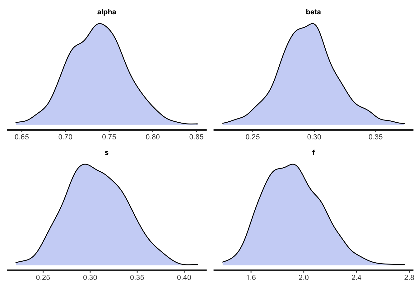
As before, our Stan model has estimated the parameter values reasonably well. If we were to run an experiment with this structure, and collect data from \(N = 50\) participants, we can be reasonably confident that this Stan model will accurately estimate our participants’ greediness and learning rate in reinforcement learning, and tendency to socially learn and conform.
References
Barrett, B. J., McElreath, R. L., & Perry, S. E. (2017). Pay-off-biased social learning underlies the diffusion of novel extractive foraging traditions in a wild primate. Proceedings of the Royal Society B, 284(1856), 20170358.
Deffner, D., Kleinow, V., & McElreath, R. (2020). Dynamic social learning in temporally and spatially variable environments. Royal Society Open Science, 7(12), 200734.
McElreath, R., Bell, A. V., Efferson, C., Lubell, M., Richerson, P. J., & Waring, T. (2008). Beyond existence and aiming outside the laboratory: estimating frequency-dependent and pay-off-biased social learning strategies. Philosophical Transactions of the Royal Society B, 363(1509), 3515-3528.
McElreath, R. (2020). Statistical rethinking: A Bayesian course with examples in R and Stan. Chapman and Hall/CRC.
McElreath R (2021). rethinking: Statistical Rethinking book package. R package version 2.21.
Sutton, R. S., & Barto, A. G. (2018). Reinforcement learning: An introduction. MIT press.
Toyokawa, W., Whalen, A., & Laland, K. N. (2019). Social learning strategies regulate the wisdom and madness of interactive crowds. Nature Human Behaviour, 3(2), 183-193.