Model 14: Social networks
Introduction
Most of the previous models assume unstructured populations in which every agent can potentially learn from any other agent. Exceptions are Model 7 (migration) and Model 11 (cultural group selection), in which agents can only learn from members of their own sub-population, and Model 10 (polarisation) in which agents are in a spatial grid and can only learn from their 4 or 8 neighbours.
Here we will extend this to explicitly model social networks of agents. Social networks specify the exact links between every agent. For example, a friendship network might capture who is friends with who within a group; a kin network might capture who is related to whom in a society; and a citation network might capture which scientists cite which other scientists in their papers. Social network analysis originates in sociology, but has become increasingly used in studies of cultural evolution in recent years.
Terminology
In the terminology of social network analysis, individuals or agents are called ‘nodes’ or ‘vertices’, and the connections between them are called ‘links’ or ‘edges’. Networks can be undirected, which is when every edge from node A to node B is mirrored by an equivalent edge from node B to node A. For example, in a kin network, if person A is related to person B, then by definition person B will also be related to person A. In contrast, a directed network can have directional links. For example, in a citation network, scientist A might cite scientist B, but scientist B might never cite scientist A. Networks can be unweighted, in which each edge is of equal strength or intensity, or weighted, in which each edge is of different strength or intensity. For example, a citation network might weight edges by the number of citations, such that if scientist A cites scientist B 10 times and scientist B cites scientist A 100 times, the latter edge is weighted higher.
Adjacency matrices
First we will write some code to generate social networks, before looking at how information spreads on those networks.
Social networks are typically represented with an adjacency matrix. For a network of \(N\) individuals, this is an \(N\) x \(N\) matrix. The \(N\) rows represent nodes from which edges originate, while the \(N\) columns represent nodes at which edges terminate. For an unweighted network, each cell contains 0 if there is no edge connecting the row and column nodes, or 1 if there is an edge between those nodes. For example, a 1 in row 3, column 5 indicates an edge coming from node 3 to node 5. Assuming nodes cannot connect to themselves, the diagonal is always full of zeroes.
This code creates an empty \(N\) x \(N\) matrix called network full of zeroes.
##       [,1] [,2] [,3] [,4] [,5] [,6] [,7] [,8] [,9] [,10]
##  [1,]    0    0    0    0    0    0    0    0    0     0
##  [2,]    0    0    0    0    0    0    0    0    0     0
##  [3,]    0    0    0    0    0    0    0    0    0     0
##  [4,]    0    0    0    0    0    0    0    0    0     0
##  [5,]    0    0    0    0    0    0    0    0    0     0
##  [6,]    0    0    0    0    0    0    0    0    0     0
##  [7,]    0    0    0    0    0    0    0    0    0     0
##  [8,]    0    0    0    0    0    0    0    0    0     0
##  [9,]    0    0    0    0    0    0    0    0    0     0
## [10,]    0    0    0    0    0    0    0    0    0     0
Technically this isn’t a network, as no-one is connected to anyone else. Let’s add some connections:
edges <- data.frame(nodeA = c(1,4,7,8,9), nodeB = c(2,7,10,1,1))

for (i in 1:5) {

  network[edges$nodeA[i], edges$nodeB[i]] <- 1
  network[edges$nodeB[i], edges$nodeA[i]] <- 1

}

network
## [,1] [,2] [,3] [,4] [,5] [,6] [,7] [,8] [,9] [,10]
## [1,] 0 1 0 0 0 0 0 1 1 0
## [2,] 1 0 0 0 0 0 0 0 0 0
## [3,] 0 0 0 0 0 0 0 0 0 0
## [4,] 0 0 0 0 0 0 1 0 0 0
## [5,] 0 0 0 0 0 0 0 0 0 0
## [6,] 0 0 0 0 0 0 0 0 0 0
## [7,] 0 0 0 1 0 0 0 0 0 1
## [8,] 1 0 0 0 0 0 0 0 0 0
## [9,] 1 0 0 0 0 0 0 0 0 0
## [10,] 0 0 0 0 0 0 1 0 0 0Here we have added five undirected edges between the pairs of nodes specified in edges. These are undirected because for every edge from node A to node B, we also create an edge between node B and node A. This makes the matrix, and every matrix containing only undirected edges, symmetrical. This can be verified using the isSymmetric command:
## [1] TRUEWeighted networks contain values other than 1, denoting the strength of the edge.
Small world networks
Watts & Strogatz (1998) introduced a simple way of generating realistic social networks. Imagine a ring of \(N\) nodes, each representing one agent. The end of the ring joins back to the first node. Think of this arrangement as the physical proximity or spatial arrangement of agents, like neighbouring houses in a big cul-de-sac.
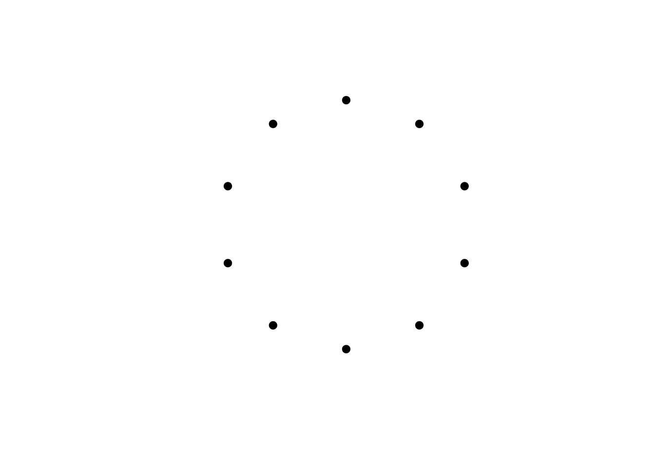
It helps to draw this ring arrangement. Here is some code to draw \(N\) points in a ring. We first create an empty plot with no labels or axes and a square aspect ratio. Then the parametric form of the equation of a circle is used to draw \(N\) evenly spaced points around the origin (0,0) (note that angles in the equation are expressed in radians not degrees).
# N agents around the origin in a big circle
plot(NULL,
     xlim = c(-5.5,5.5),
     ylim = c(-5.5,5.5),
     xlab = "",
     ylab = "",
     axes = FALSE,
     asp = 1)

for (i in 1:N) {

  points(5*sin((i-1)*2*pi/N), 5*cos((i-1)*2*pi/N),
         pch = 16,
         cex = 1.2)

}
We now add edges to represent social ties within this spatial arrangement. Watts & Strogatz (1998) assume first that each node is connected to \(k\) neighbouring nodes, \(k/2\) to the left and \(k/2\) to the right (\(k\) must therefore be an even number).
The following code generates an adjacency matrix for \(k = 4\). We cycle through each row / node of the matrix, and for each one assign 1 to its \(k/2\) neighbours to the right, and \(k/2\) neighbours to the left. Because the ring joins round back to the beginning, if the neighbour column is greater than \(N\) then we subtract \(N\), and if it’s less than 1 then we add \(N\), to wrap around to the other side.
k <- 4

# create empty adjacency matrix
network <- matrix(0, nrow = N, ncol = N, )

# create ring lattice network
for (Row in 1:N) {

  # k/2 neighbours to the right
  Col <- (Row+1):(Row+k/2)
  Col[which(Col > N)] <- Col[which(Col > N)] - N
  network[Row, Col] <- 1

  # k/2 neighbours to the left
  Col <- (Row-k/2):(Row-1)
  Col[which(Col < 1)] <- Col[which(Col < 1)] + N
  network[Row, Col] <- 1

}

network
## [,1] [,2] [,3] [,4] [,5] [,6] [,7] [,8] [,9] [,10]
## [1,] 0 1 1 0 0 0 0 0 1 1
## [2,] 1 0 1 1 0 0 0 0 0 1
## [3,] 1 1 0 1 1 0 0 0 0 0
## [4,] 0 1 1 0 1 1 0 0 0 0
## [5,] 0 0 1 1 0 1 1 0 0 0
## [6,] 0 0 0 1 1 0 1 1 0 0
## [7,] 0 0 0 0 1 1 0 1 1 0
## [8,] 0 0 0 0 0 1 1 0 1 1
## [9,] 1 0 0 0 0 0 1 1 0 1
## [10,] 1 1 0 0 0 0 0 1 1 0We can update our plotting code to add these edges, again using the equation of a circle. We also wrap it in a self-contained function to re-use later.
DrawNetwork <- function(network) {

  # get N from network matrix
  N <- ncol(network)

  # N agents around the origin in a big circle
  plot(NULL,
       xlim = c(-5.5,5.5),
       ylim = c(-5.5,5.5),
       xlab = "",
       ylab = "",
       axes = FALSE,
       asp = 1)

  for (i in 1:N) {

    points(5*sin((i-1)*2*pi/N), 5*cos((i-1)*2*pi/N),
           pch = 16,
           cex = 1.2)

  }

  # lines representing edges
  for (i in 1:N) {

    for (j in which(network[i,] == 1)) {

      lines(x = c(5*sin((i-1)*2*pi/N), 5*sin((j-1)*2*pi/N)),
            y = c(5*cos((i-1)*2*pi/N), 5*cos((j-1)*2*pi/N)))

    }

  }

}

DrawNetwork(network)
So far so straightforward: each node is connected to its four immediate neighbours. Real social networks, however, have additional connections. Some people might be friends with someone across the other side of the cul-de-sac, and never speak to their physical neighbours. Some scientists might collaborate with other scientists in different countries, or different academic disciplines.
Therefore with probability \(p\) the above network is ‘rewired’. We cycle through each node from 1 to \(N\). For each one, we take the first neighbour to its right, which given that \(k >= 2\) it will be connected to with an edge. Then, with probability \(p\), we pick a new_neighbour randomly from the set of all nodes excluding self and nodes to which connections already exist. The existing edge is removed, and a new edge is drawn to the new_neighbour. Remember, this is an undirected network, so every change made from node A to node B needs to be repeated for node B to node A. This keeps the matrix symmetrical. Finally, this whole process is repeated for the next connected neighbour, up to the last, so \(k / 2\) times in total.
p <- 0.2

# rewiring via p

for (j in 1:(k/2)) {

  for (i in 1:N) {

    if (runif(1) < p) {

      # pick jth clockwise neighbour
      neighbour <- i + j
      if (neighbour > N) neighbour <- neighbour - N

      # pick random new neighbour, excluding self and duplicate edges
      new_neighbour <- which(network[i,] == 0)
      new_neighbour <- new_neighbour[new_neighbour != i]
      new_neighbour <- sample(new_neighbour, 1)

      # remove edge to old neighbour
      network[i,neighbour] <- 0
      network[neighbour,i] <- 0

      # make edge to new neighbour
      network[i, new_neighbour] <- 1
      network[new_neighbour, i] <- 1

    }

  }

}

network
## [,1] [,2] [,3] [,4] [,5] [,6] [,7] [,8] [,9] [,10]
## [1,] 0 0 1 1 0 0 0 0 1 1
## [2,] 0 0 1 1 0 0 0 0 0 0
## [3,] 1 1 0 1 0 0 1 0 0 0
## [4,] 1 1 1 0 1 1 0 0 0 1
## [5,] 0 0 0 1 0 1 1 0 0 0
## [6,] 0 0 0 1 1 0 1 1 0 0
## [7,] 0 0 1 0 1 1 0 1 1 0
## [8,] 0 0 0 0 0 1 1 0 1 1
## [9,] 1 0 0 0 0 0 1 1 0 1
## [10,] 1 0 0 1 0 0 0 1 1 0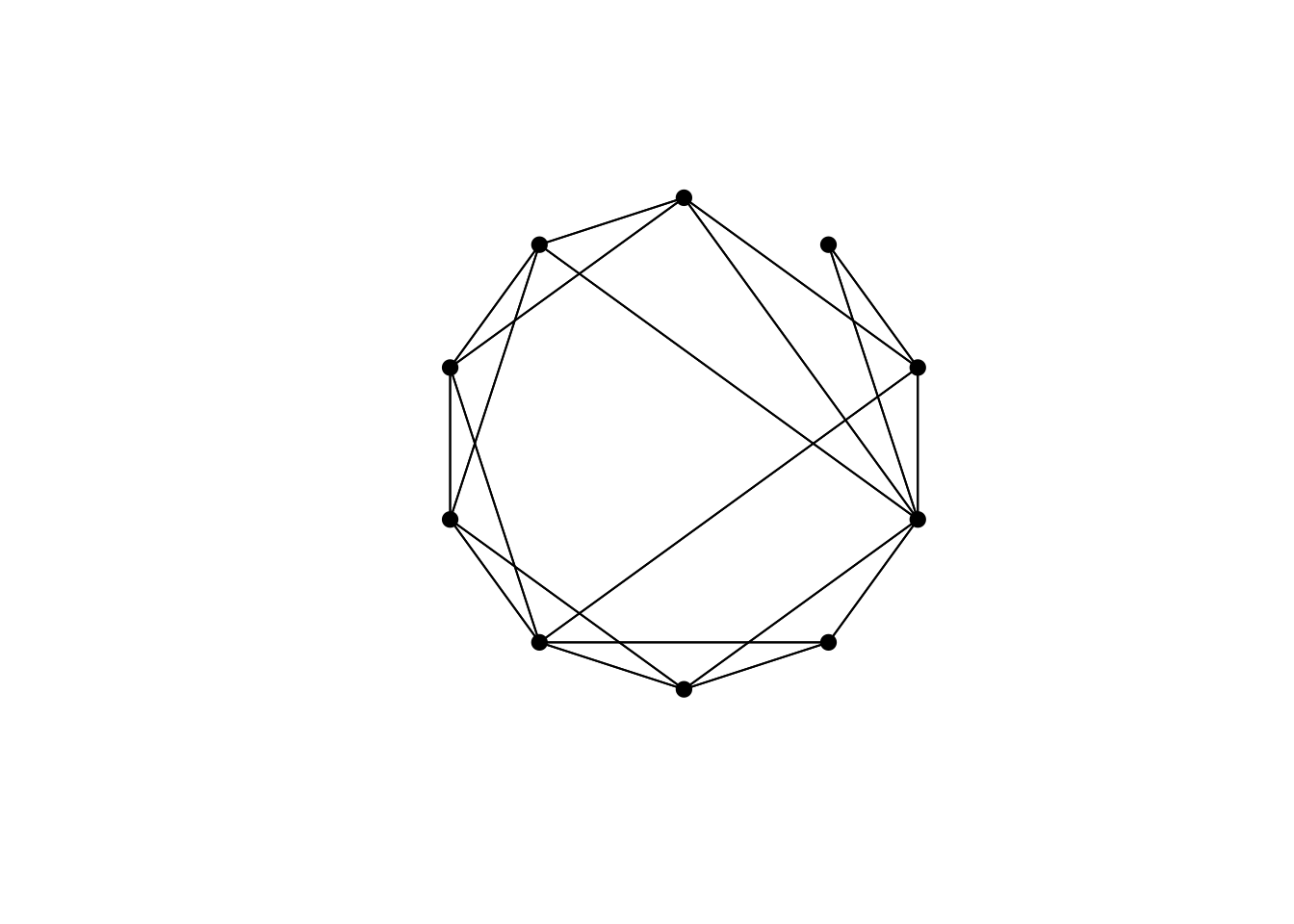
The resulting network is still mostly clustered, like the original network, but has a few long edges connecting otherwise distant nodes. Watts & Strogatz (1998) called this a ‘small world network’, after the phenomenon by which surprisingly few connections link any two people in a typical social network. The most famous example is the six degrees of Kevin Bacon, where any actor can be connected to Kevin Bacon via shared movie credits in six steps or less. Watts & Strogatz (1998) showed formally that their small world network algorithm adequately captures the characteristics of various real-world networks, including film actors.
We wrap the above code in a function to more easily re-run it with different parameter values, and re-use it later.
SmallWorld <- function(N, k, p, draw_plot = TRUE) {
# 1. create empty adjacency matrix
network <- matrix(0, nrow = N, ncol = N, )
# 2. create ring lattice network
for (Row in 1:N) {
# k/2 neighbours to the right
Col <- (Row+1):(Row+k/2)
Col[which(Col > N)] <- Col[which(Col > N)] - N
network[Row, Col] <- 1
# k/2 neighbours to the left
Col <- (Row-k/2):(Row-1)
Col[which(Col < 1)] <- Col[which(Col < 1)] + N
network[Row, Col] <- 1
}
# 3. rewiring via p
for (j in 1:(k/2)) {
for (i in 1:N) {
if (runif(1) < p) {
# pick jth clockwise neighbour
neighbour <- i + j
if (neighbour > N) neighbour <- neighbour - N
# pick random new neighbour, excluding self and duplicate edges
new_neighbour <- which(network[i,] == 0)
new_neighbour <- new_neighbour[new_neighbour != i]
new_neighbour <- sample(new_neighbour, 1)
# remove edge to old neighbour
network[i,neighbour] <- 0
network[neighbour,i] <- 0
# make edge to new neighbour
network[i, new_neighbour] <- 1
network[new_neighbour, i] <- 1
}
}
}
# 4. draw network if draw_network == TRUE
if (draw_plot == TRUE) {
DrawNetwork(network)
}
# output network from function
network
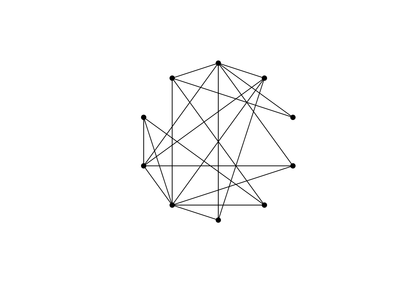
}Increasing \(p\) to 1 gives a fully random network, with every original edge rewired:
Increasing \(N\) to 40 and setting \(p = 0.1\) gives a typical small world network:
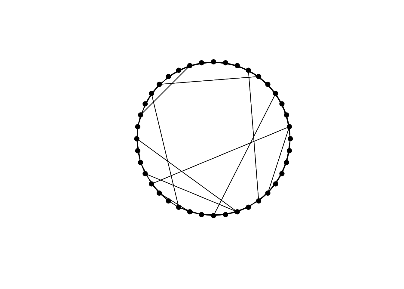
Most edges are still connecting adjacent nodes in the ring, but a small number of long ties traverse the ring connecting otherwise-distant nodes.
Network properties: Path length and clustering
The reason small world networks with a small but non-zero \(p\) like the one above are interesting is because they are clustered yet also have short path lengths. A path between two nodes is the set of edges linking those nodes. Path length is the number of edges in that path. The shortest path length is the minimum number of edges connecting two nodes. Two nodes directly connected by an edge have a shortest path length of 1; two nodes not directly connected but connected via a third node have shortest path length of 2; and so on.
Small world networks have much lower shortest path lengths than fully clustered \(p = 0\) networks because of the long ties linking distant parts of the network. This is of importance to social learning and cultural evolution, because if we assume that information flows along edges, then small world networks will be much more efficient at spreading information across the whole network than fully clustered (\(p = 0\)) networks. We will explore this formally later, but for now let’s quantitatively measure path length to confirm the above claims.
The following function get_path_length calculates, for a given network, the shortest path length between node A and node B. The code is a little opaque, but essentially it maintains a set \(v\) of nodes that are increasing degrees to A (degree 0 is node A itself, degree 1 are the nodes connected to A by one edge, degree 2 the nodes connected to A by two edges, etc.), and if any of the nodes in \(v\) are B, the loop breaks and the current path_length is returned.
get_path_length <- function(network, A, B) {

  path_length <- NA
  N <- ncol(network)

  # start with vertex v = A
  v <- A

  for (i in 1:(N-1)) {

    # if any vertices v are connected to B, set path_length and break
    if (any(network[v,B] == 1)) {

      path_length <- i
      break

    }

    # otherwise, new v is the vertices connected to previous v
    v <- which(as.matrix(network[,v] == 1), arr.ind = T)[,1]

  }

  # return path_length
  path_length

}
Some examples for the previous network generated above:
## [1] 1## [1] 6## [1] 1The function get_mean_path_length below calculates the average path length between every possible pair of nodes, and calculates this for network:
get_mean_path_length <- function(network) {

  mean_path_length <- 0
  N <- ncol(network)

  for (i in 1:(N-1)) {

    for (j in (i+1):N) {

      mean_path_length <- mean_path_length + get_path_length(network,i,j)

    }

  }

  mean_path_length / (N*(N-1)/2)

}

get_mean_path_length(network)
## [1] 1.6Let’s use this function to plot mean path length \(L\) against \(p\), averaging across \(r_{max}\) runs for each value of \(p\):
p <- seq(0, 1, 0.1)
L <- rep(0, length(p))
r_max <- 10

for (r in 1:r_max) {

  for (i in 1:length(p)) {

    L[i] <- L[i] + get_mean_path_length(SmallWorld(40, 4, p[i], draw_plot = F))

  }

}

# average over all runs
L <- L / r_max

# plot L vs p
plot(x = p,
     y = L,
     type = 'l',
     ylab = "mean shortest path length, L",
     xlab = "rewiring probability, p")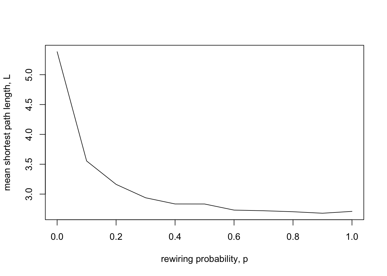
As expected, as networks increase in long ties, mean path length gets shorter, from 5.38 at \(p = 0\) to around 2.7 for \(p = 0.5\) and above. Note that the biggest drop occurs for small values of \(p\). Only a small amount of rewiring (\(p = 0.1\)) is needed to cause mean path length to reduce considerably. In contrast, increasing \(p\) from 0.5 to 1 has little effect. Once there are a few long ties connecting different parts of the ring, further long ties are redundant.
Clustering refers to the cliqueishness of a particular neighbourhood within the network. The clustering coefficient for node \(i\) is defined as, for all neighbours directly connected to node \(i\), the proportion of all possible edges linking those neighbours to each other that are actually present. For example, if node \(i\) has edges to \(k_i = 3\) neighbours, there are a maximum of \(k_i(k_i - 1)/2 = 3\) potential edges between those three neighbours (between neighbour A & B, A & C, and B & C). Say only two of these edges are actually present (e.g. between A & B and A & C), then the clustering coefficient is 2/3.
The function get_clustering_coef below calculates the clustering coefficient for a specific node in the adjacency matrix network. First we get the set of directly connected neighbours. Then we create a mini-adjacency-matrix containing just those neighbours. Then we count the number of edges between them, and divide by all possible edges. Note that we use the function upper.tri() to get the sum of all edges in only one half of the matrix, given that our network is undirected. The clustering coefficient for node 10 is shown as an example.
get_clustering_coef <- function(network, node) {

  # get direct neighbours of node
  neighbours <- which(network[node,] == 1)

  # number of neighbours
  k_i <- length(neighbours)

  # create mini-matrix representing neighbours
  neighbours <- network[neighbours, neighbours]

  # count edges, ignoring duplicates given that network is undirected
  # and divide by all possible edges
  sum(neighbours[upper.tri(neighbours)] == 1) / (k_i*(k_i-1)/2)

}

get_clustering_coef(network, 10)
## [1] 0.5Now we can get the mean clustering coefficient across all \(N\) nodes using another function, and use it to calculate this for network:
get_mean_clustering_coef <- function(network) {

  mean_clustering_coef <- 0
  N <- ncol(network)

  for (i in 1:N) {

    mean_clustering_coef <- mean_clustering_coef + get_clustering_coef(network, i)

  }

  # return mean clustering coefficient
  mean_clustering_coef / N

}

get_mean_clustering_coef(network)
## [1] 0.5066667And finally, as for path length, we can plot clustering coefficient \(C\) for a range of \(p\):
p <- seq(0, 1, 0.1)
C <- rep(0, length(p))
r_max <- 10

for (r in 1:r_max) {

  for (i in 1:length(p)) {

    C[i] <- C[i] + get_mean_clustering_coef(SmallWorld(40, 4, p[i], draw_plot = F))

  }

}

# average over all runs
C <- C / r_max

# plot L vs p
plot(x = p,
     y = C,
     type = 'l',
     ylab = "mean clustering coefficient, C",
     xlab = "rewiring probability, p")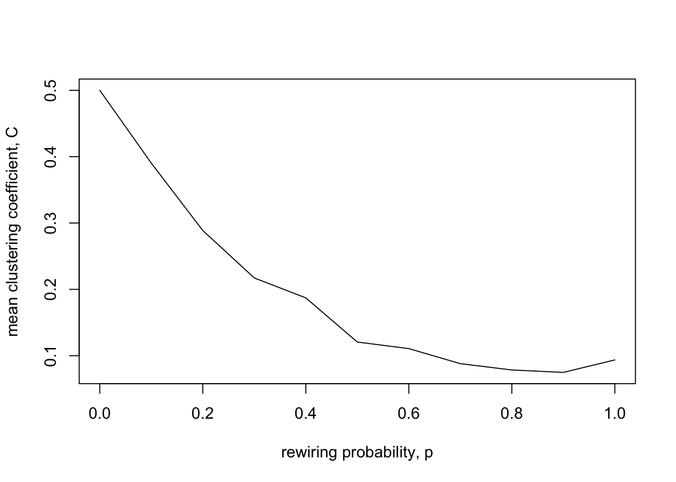
As for path length, the clustering coefficient drops as \(p\) increases and networks get more randomised. This makes sense, as randomisation will break up clusters of densely connected neighbours. Note however that the clustering coefficient drops less sharply than path length. This means that, for reasonably small values of \(p\) (e.g. \(p = 0.1\) for the \(N\) and \(k\) shown above), i.e. in the ‘small world’ region in between fully clustered and fully random, the network retains most of its clustering but has much reduced path length.
Model 14
Now we have a way of generating social networks, we can simulate the spread of information in those networks. We adapt the SImodel from Model 13a in which \(N\) initially Susceptible (\(S\)) agents are seeded with a small number of Infected (\(I\)) agents. Whereas previously the Infection (i.e. the cultural trait) spread through an unstructured population, now it spreads along the edges in a network created using SmallWorld.
First we create a vector of \(N\) agents all initially with trait \(S\). For reasons that will become apparent later, rather than randomly setting a proportion \(I_0\) of agents to \(I\) as in SImodel, we make the first \(I_0\) agents in agent \(I\). Note that \(I_0\) is now a positive integer, rather than a probability.
N <- 40
I_0 <- 2

# create first generation of agents
agent <- rep("S", N)

# add I_0 adjacent infected agents
agent[1:I_0] <- "I"

agent
## [1] "I" "I" "S" "S" "S" "S" "S" "S" "S" "S" "S" "S" "S" "S" "S" "S" "S" "S" "S"
## [20] "S" "S" "S" "S" "S" "S" "S" "S" "S" "S" "S" "S" "S" "S" "S" "S" "S" "S" "S"
## [39] "S" "S"We also create a network for our \(N\) agents using SmallWorld:
Now we pick focal \(S\) agents in random order to potentially be infected by (i.e. socially learn from) \(I\) individuals. For each focal, we get that focal’s neighbours to which they are connected via edges. Then, if at least \(n\) of those neighbours are \(I\), the focal becomes \(I\). For now, we set \(n = 1\), so only one neighbour needs to be \(I\) in order to spread the trait.
n <- 1

# randomly ordered susceptible focals
focal <- sample(which(agent == "S"))

# cycle through focals
for (i in focal) {

  # get i's neighbours
  neighbours <- which(network[i,] == 1)

  # if at least one neighbour is I, adopt I
  if (sum(agent[neighbours] == "I") >= n) {

    agent[i] <- "I"

  }

}

agent
## [1] "I" "I" "I" "I" "I" "S" "S" "S" "S" "S" "S" "S" "S" "S" "S" "S" "S" "S" "S"
## [20] "S" "S" "S" "S" "S" "S" "S" "S" "S" "S" "S" "S" "S" "S" "S" "S" "S" "S" "S"
## [39] "I" "I"You should see that several agents have flipped to \(I\) as a result of contagion on the network.
Let’s wrap up the above code into a function Contagion which contains loops for timesteps and independent runs, records the frequency of \(I\) in an output dataframe, and plots this frequency.
Contagion <- function(N, k, p, n, I_0, t_max, r_max) {

  # create a matrix with t_max rows and r_max columns, fill with NAs, convert to dataframe
  output <- as.data.frame(matrix(NA, t_max, r_max))

  # purely cosmetic: rename the columns with run1, run2 etc.
  names(output) <- paste("run", 1:r_max, sep="")

  for (r in 1:r_max) {

    # create first generation of agents
    agent <- rep("S", N)

    # add I_0 adjacent infected agents
    agent[1:I_0] <- "I"

    # add first generation's p to first row of column run
    output[1,r] <- sum(agent == "I") / N

    # create network for agent
    network <- SmallWorld(N, k, p, draw_plot = F)

    for (t in 2:t_max) {

      # randomly ordered susceptible focals
      focal <- sample(which(agent == "S"))

      # cycle through focals
      for (i in focal) {

        # get i's neighbours
        neighbours <- which(network[i,] == 1)

        # if at least one neighbour is I, adopt I
        if (sum(agent[neighbours] == "I") >= n) {

          agent[i] <- "I"

        }

      }

      output[t,r] <- sum(agent == "I") / N

    }

  }

  # first plot a thick line for the mean proportion of I
  plot(rowMeans(output),
       type = 'l',
       ylab = "proportion of Infected agents",
       xlab = "generation",
       ylim = c(0,1),
       lwd = 3,
       main = paste("N = ", N,
                    ", k = ", k,
                    ", p = ", p,
                    ", n = ", n,
                    ", I_0 = ", I_0,
                    sep = ""))

  for (r in 1:r_max) {

    # add lines for each run, up to r_max
    lines(output[,r], type = 'l')

  }

  # export output
  output

}
Because information spreads too fast to be interesting on small networks of \(N = 40\), we increase the population size to \(N = 1000\). First, what happens in a completely clustered \(p = 0\) network with no long ties?
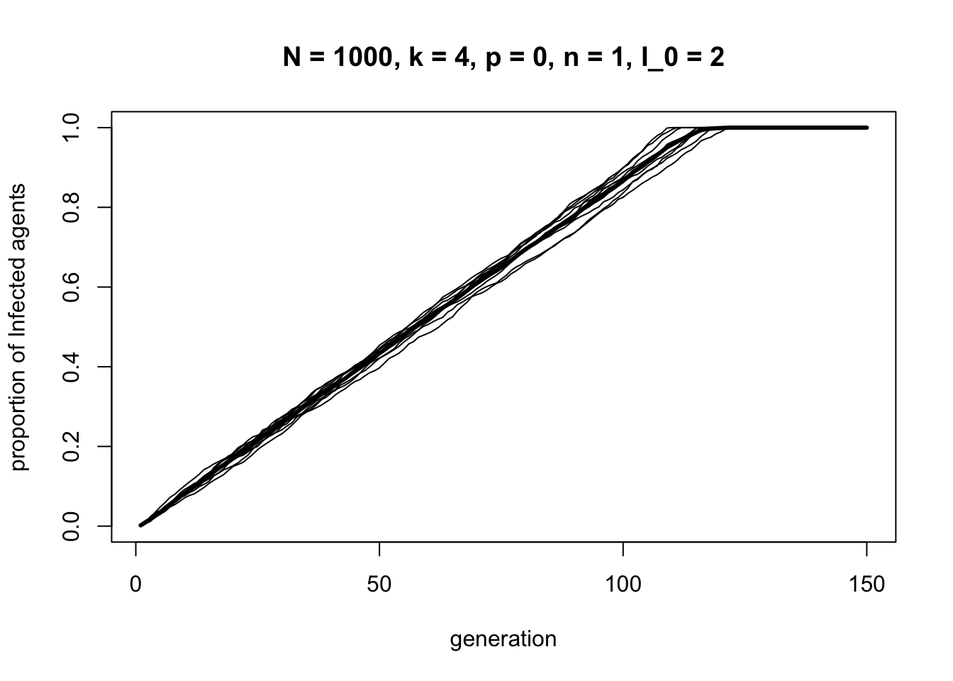
In a clustered network information spreads at a constant rate node-by-node around the ring network until it reaches every node at around timestep 120.
Now let’s try a small world network, \(p = 0.01\)
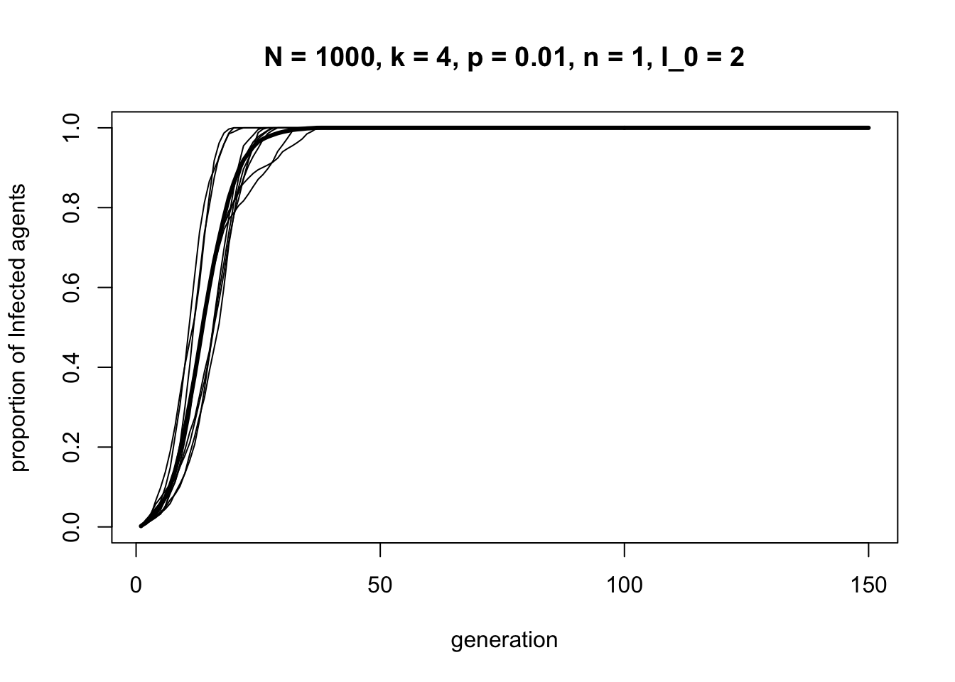
In a small world network with just a small number of long ties (approximately \(Np = 10\)), information spreads much, much faster. It flows along the shortcuts across the ring, not needing to travel node-by-node around the ring.
We can see this more clearly in the following four-panel plot, comparing \(p\) = 0, 0.001, 0.01 and 0.1:
# 2 rows, 2 columns
par(mfrow=c(2,2))

# p = 0
panel1 <- Contagion(N = 1000,
                    k = 4,
                    p = 0,
                    n = 1,
                    I_0 = 2,
                    t_max = 150,
                    r_max = 5)

# p = 0.001
panel2 <- Contagion(N = 1000,
                    k = 4,
                    p = 0.001,
                    n = 1,
                    I_0 = 2,
                    t_max = 150,
                    r_max = 5)

# p = 0.01
panel3 <- Contagion(N = 1000,
                    k = 4,
                    p = 0.01,
                    n = 1,
                    I_0 = 2,
                    t_max = 150,
                    r_max = 5)

# p = 0.1
panel4 <- Contagion(N = 1000,
                    k = 4,
                    p = 0.1,
                    n = 1,
                    I_0 = 2,
                    t_max = 150,
                    r_max = 5)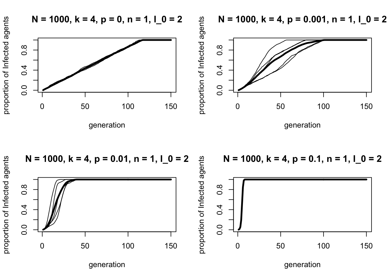
As \(p\) increases by each order of magnitude, information spreads ever faster.
What happens if we increase \(n\) from 1 to 2? Now, at least two neighbours need to be \(I\) in order for the focal \(S\) agent to convert to \(I\).
# 2 rows, 2 columns
par(mfrow=c(2,2))

# p = 0
panel1 <- Contagion(N = 1000,
                    k = 4,
                    p = 0,
                    n = 2,
                    I_0 = 2,
                    t_max = 350,
                    r_max = 5)

# p = 0.001
panel2 <- Contagion(N = 1000,
                    k = 4,
                    p = 0.001,
                    n = 2,
                    I_0 = 2,
                    t_max = 350,
                    r_max = 5)

# p = 0.01
panel3 <- Contagion(N = 1000,
                    k = 4,
                    p = 0.01,
                    n = 2,
                    I_0 = 2,
                    t_max = 350,
                    r_max = 5)

# p = 0.1
panel4 <- Contagion(N = 1000,
                    k = 4,
                    p = 0.1,
                    n = 2,
                    I_0 = 2,
                    t_max = 350,
                    r_max = 5)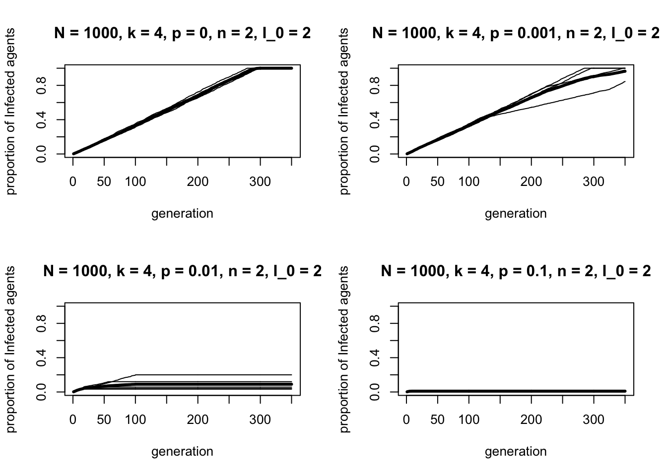
Increasing \(p\) when \(n = 2\) has the opposite effect to \(n = 1\): the proportion of \(I\) agents decreases as \(p\) increases. For \(p = 0.1\), the trait hardly spreads at all.
This is because long ties generated when \(p > 0\) break up clusters of \(I\) nodes that are needed when \(n = 2\). In a highly clustered network, groups of \(I\) nodes emerge, each one providing at least two \(I\) neighbours for neighbouring \(S\) nodes to be converted. When some of those local ties are diverted to another part of the ring via rewiring, these clusters of \(I\) are less likely to remain. Ties to another part of the network are no good because they will divert to a region full of \(S\)s 1.
This phenomenon was called ‘complex contagion’ in an influential paper by Centola et al. (2007), in contrast to ‘simple contagion’ when \(n = 1\). Simple contagions that require just a single demonstrator to spread are facilitated by the long ties in small world networks. Examples of simple contagions might be the spread of news stories (‘JFK has been shot’), sports results (‘Watford beat Liverpool’) or job openings (‘the coffee shop is hiring’). Simple contagion is also most similar to disease contagion: exposure to just one person with covid can make you catch covid.
Complex contagions, however, require exposure to multiple demonstrators to successfully spread. Examples might be political or social movements, unproven new technologies or methods of contraception. Centola (2010) demonstrated experimentally that health behaviours spread further and faster on clustered networks than random networks with lots of long ties because of the need for exposure to multiple demonstrators.
Summary
Social networks capture the social ties between each individual in a population, going beyond the unstructured or weakly structured populations of previous models. Here we explored small world networks, a class of network that vary from highly clustered to highly random. In between these two extremes are networks that remain clustered but contain a small number of long ties connecting distant parts of the network. These small world networks are representative of many real world human social networks. Most of our friends and colleagues are local, but we also probably have a few long-distance acquaintances who connect us to more distant individuals.
For simple contagions which require minimal exposure to a single demonstrator to cause the adoption of a trait, small world networks with more long ties are beneficial. These long ties quickly propel information to all parts of the network. For complex contagions which require exposure to multiple demonstrators, however, long ties can prevent transmission by breaking up local clusters. This shows an important interaction between network topology and cultural trait transmission dynamics.
For further work that explicitly links cultural evolution and social networks, see Cantor et al. (2021), who examined how the diffusion of cultural traits is affected by several other kinds of networks beyond the small world networks examined above; Migliano et al. (2017), who measured the social networks of Agta and BaYaka hunter gatherers and explored how these networks affect cultural diffusion; and Smolla & Akçay (2019), who modelled how cultural selection for skill specialisation can shape social network structure.
In terms of programming, we learned how to use adjacency matrices to capture the edges between each node in a network. This allowed us to use R’s built-in matrix functions such as isSymmetric to test whether a network is undirected, and lower.tri / upper.tri to select just the in or out nodes. We also learned how to draw a network using the standard plot, points and lines functions plus a bit of circle geometry, and use adjacency matrices to calculate path lengths and clustering coefficients. There are R packages that do all these things and much more, the most popular being igraph. While it is absolutely fine to use such packages, it is often easier to understand exactly what a measure means, or what an algorithm is doing, if we code it from scratch.
Exercises
Play around with different values of \(N\), \(k\), \(p\), \(I_0\) and \(n\) in Contagion. Under what combinations of parameter values does the ‘complex contagion’ effect occur, i.e. increasing \(p\) reduces diffusion of the trait when \(n > 1\)? Why?
Rewrite the DrawNetwork function such that filled points indicate \(I\) agents and unfilled points indicate \(S\) agents. Similar to how we did for Model 10 (polarisation), modify Contagion to draw the network at prespecified timesteps (e.g. \(t = 1, 50, 100, 150\)) to visualise how the \(I\) trait spreads.
Rewrite SmallWorld to create a network on a square lattice rather than a ring lattice. Parameter \(k\) should now be the number of Moore or von Neumann neighbours to whom edges connect. How do simple and complex contagion differ on a square lattice?
References
Cantor, M., Chimento, M., Smeele, S. Q., He, P., Papageorgiou, D., Aplin, L. M., & Farine, D. R. (2021). Social network architecture and the tempo of cumulative cultural evolution. Proceedings of the Royal Society B, 288(1946), 20203107.
Centola, D., & Macy, M. (2007). Complex contagions and the weakness of long ties. American Journal of Sociology, 113(3), 702-734.
Centola, D. (2010). The spread of behavior in an online social network experiment. Science, 329(5996), 1194-1197.
Migliano, A. B., Page, A. E., Gómez-Gardeñes, J., Salali, G. D., Viguier, S., Dyble, M., … & Vinicius, L. (2017). Characterization of hunter-gatherer networks and implications for cumulative culture. Nature Human Behaviour, 1(2), 1-6.
Smolla, M., & Akçay, E. (2019). Cultural selection shapes network structure. Science Advances, 5(8), eaaw0609.
Watts, D. J., & Strogatz, S. H. (1998). Collective dynamics of ‘small-world’ networks. Nature, 393(6684), 440-442.
Note that this is why initially we make \(I_0\) adjacent nodes \(I\) rather than a proportion \(I_0\), because it is highly unlikely that the latter will lead to two or more adjacent \(I\) nodes, and when \(n = 2\) the trait will never spread even for \(p = 0\).↩︎