Model 7: Migration
Introduction
Along with selection, mutation and drift, another fundamental driver of genetic evolution is migration. The same is true of cultural evolution. Migration has been a permanent fixture of our species since we first dispersed out of Africa. The movement of people from group to group can shape between-group cultural diversity, and spread beneficial technologies or ideas from group to group.
Model 7
In Model 7 we will examine the effect of migration on between-group diversity. Previous models all featured a single group of agents. Now that we are interested in migration, we need to simulate multiple groups. Let’s keep things simple and add one other group, making two in total: group 1 and group 2. As before, each group has \(N\) individuals in it.
As before, let’s assume that there are two traits, \(A\) and \(B\). We’ll assume for now that they are neutral, i.e. not subject to selection / biased transmission. We assume that, initially, every member of group 1 has \(A\), and every member of group 2 has \(B\). Hence, in generation 1, \(p = 1\), and \(q = 0\), where \(p\) denotes the frequency of trait \(A\) in group \(1\) and \(q\) denotes the frequency of trait \(A\) in group 2. Such a case of maximum group difference might seem extreme, but is not too far from a situation where everyone in one society speaks one language and everyone in another society speaks another language, or everyone in one group practices one religion and everyone in another practices a different religion. In any case, remember that models are simplified, extreme cases designed to check the logic of verbal arguments, not exact recreations of reality.
The following code creates two agent dataframes, one for each group, and populates them with agents according to starting frequencies \(p_0 = 1\) and \(q_0 = 0\). Unlike before, we create another column recording which group this is, 1 or 2. We then combine the two dataframes into a single one using the rbind command, which combines dataframes by rows. Finally, we check it worked by calling the first five agents in group 1, i.e. agents one to five, who should all have trait \(A\), and the first five agents in group 2, i.e. agents \(N+1\) to \(N+5\), who should all have trait \(B\).
N <- 100
p_0 <- 1
q_0 <- 0

# create first generation of group 1
agent1 <- data.frame(trait = sample(c("A","B"), N, replace = TRUE,
                     prob = c(p_0,1-p_0)),
                     group = 1)

# create first generation of group 2
agent2 <- data.frame(trait = sample(c("A","B"), N, replace = TRUE,
                     prob = c(q_0,1-q_0)),
                     group = 2)

# combine agent1 and agent2 into a single agent dataframe
agent <- rbind(agent1,agent2)

agent[1:5,]
## trait group
## 1 A 1
## 2 A 1
## 3 A 1
## 4 A 1
## 5 A 1## trait group
## 101 B 2
## 102 B 2
## 103 B 2
## 104 B 2
## 105 B 2We can also calculate the frequency of \(A\) in groups 1 and 2, i.e. \(p\) and \(q\), and check that \(p = 1\) and \(q = 0\), with this code:
p <- sum(agent$trait[agent$group == 1] == "A") / N
q <- sum(agent$trait[agent$group == 2] == "A") / N

paste("p =", p)
## [1] "p = 1"## [1] "q = 0"This code uses subsetting to get the number of \(A\)s in group 1, and then in group 2, and divides both by \(N\) to get a proportion.
Now for migration. In each timestep, we assume that each agent has a probability \(m\) of migrating. There is a problem, though. Because this is stochastic, this might result in the groups changing size. Maybe in one generation five agents move from group 1 to group 2, while only two move from group 2 to group 1. Then, group 1 would be smaller than group 2, and neither would be \(N\). This gets complicated to model, as the size of the dataframes holding agents would need to change during the simulations.
To avoid \(N\) from changing during the simulation, we can do the following, drawing inspiration from what’s known as Wright’s Island Model from population genetics. First, each agent migrates with probability \(m\), ignoring group membership. On average, this gives \(2 N m\) migrants across the entire population, given that there are two groups of \(N\) agents. We take the migrants out of their groups, leaving empty slots where they used to be. Then we put these migrants back into the empty slots at random, ignoring which group the slot is in. This keeps \(N\) constant: for every empty slot, there is a migrating agent. Some might go back into their original group, but this won’t change anything so it doesn’t really matter.
Finally, we are assuming that agents take their traits with them, for now. We will change this later.
The following code simulates one bout of migration, i.e. one generation in the model.
m <- 0.1

# 2N probabilities, one for each agent, to compare against m
probs <- runif(1:(2*N))

# with prob m, add an agent's trait to list of migrants
migrants <- agent$trait[probs < m]

# put migrants randomly into empty slots
agent$trait[probs < m] <- sample(migrants, length(migrants))

p <- sum(agent$trait[agent$group == 1] == "A") / N
q <- sum(agent$trait[agent$group == 2] == "A") / N

paste("p =", p)
## [1] "p = 0.95"## [1] "q = 0.05"You should see here that \(p\) has decreased slightly to be less than 1, and \(q\) has increased slightly to be greater than 0. Migration seems to be bringing the frequencies closer together.
The following function simply repeats the above over \(t_{max}\) generations and plots \(p\) and \(q\), all within a single function, similar to previous models. We omit multiple runs and \(r_{max}\), for brevity.
Migration <- function (N, p_0, q_0, m, t_max) {

  # create output dataframe to hold t_max values of p and q
  output <- data.frame(p = rep(NA, t_max), q = rep(NA, t_max))

  # create first generation of group 1
  agent1 <- data.frame(trait = sample(c("A","B"), N, replace = TRUE,
                       prob = c(p_0,1-p_0)),
                       group = 1)

  # create first generation of group 2
  agent2 <- data.frame(trait = sample(c("A","B"), N, replace = TRUE,
                       prob = c(q_0,1-q_0)),
                       group = 2)

  # combine agent1 and agent2 into a single agent dataframe
  agent <- rbind(agent1,agent2)

  # store first generation frequencies
  output$p[1] <- sum(agent$trait[agent$group == 1] == "A") / N
  output$q[1] <- sum(agent$trait[agent$group == 2] == "A") / N

  for (t in 2:t_max) {

    # migration

    # 2N probabilities, one for each agent, to compare against m
    probs <- runif(1:(2*N))

    # with prob m, add an agent's trait to list of migrants
    migrants <- agent$trait[probs < m]

    # put migrants randomly into empty slots
    agent$trait[probs < m] <- sample(migrants, length(migrants))

    # store frequencies in output slot t
    output$p[t] <- sum(agent$trait[agent$group == 1] == "A") / N
    output$q[t] <- sum(agent$trait[agent$group == 2] == "A") / N

  }

  plot(x = 1:nrow(output), y = output$p,
       type = 'l',
       col = "orange",
       ylab = "proportion of agents with trait A",
       xlab = "generation",
       ylim = c(0,1),
       main = paste("N = ", N, ", m = ", m, sep = ""))

  lines(x = 1:nrow(output), y = output$q, col = "royalblue")

  legend("topright",
         legend = c("p (group 1)", "q (group 2)"),
         lty = 1,
         col = c("orange", "royalblue"),
         bty = "n")

  output  # export data from function
}
Now we can run the function with a reasonably strong migration rate of \(m = 0.1\):
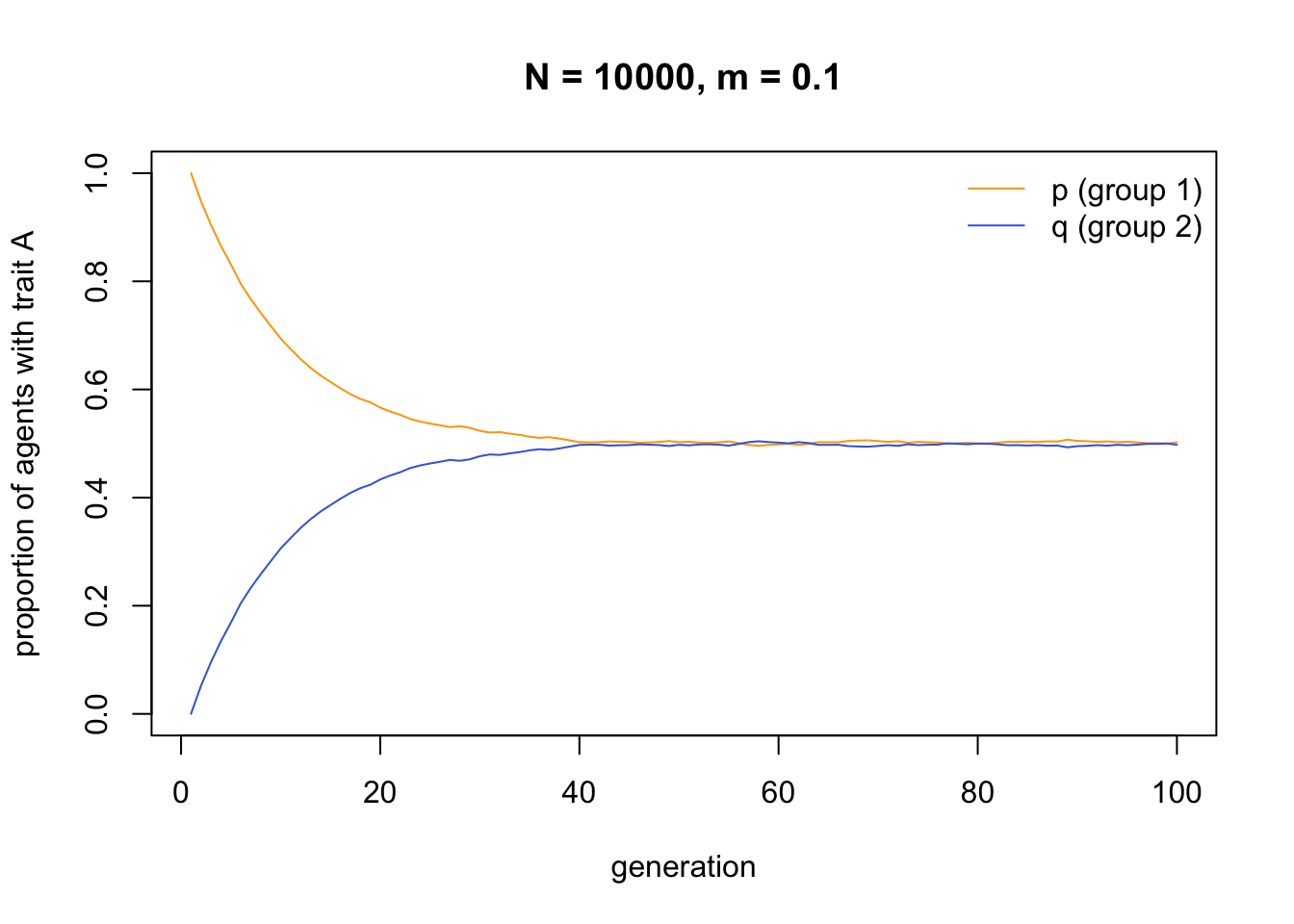
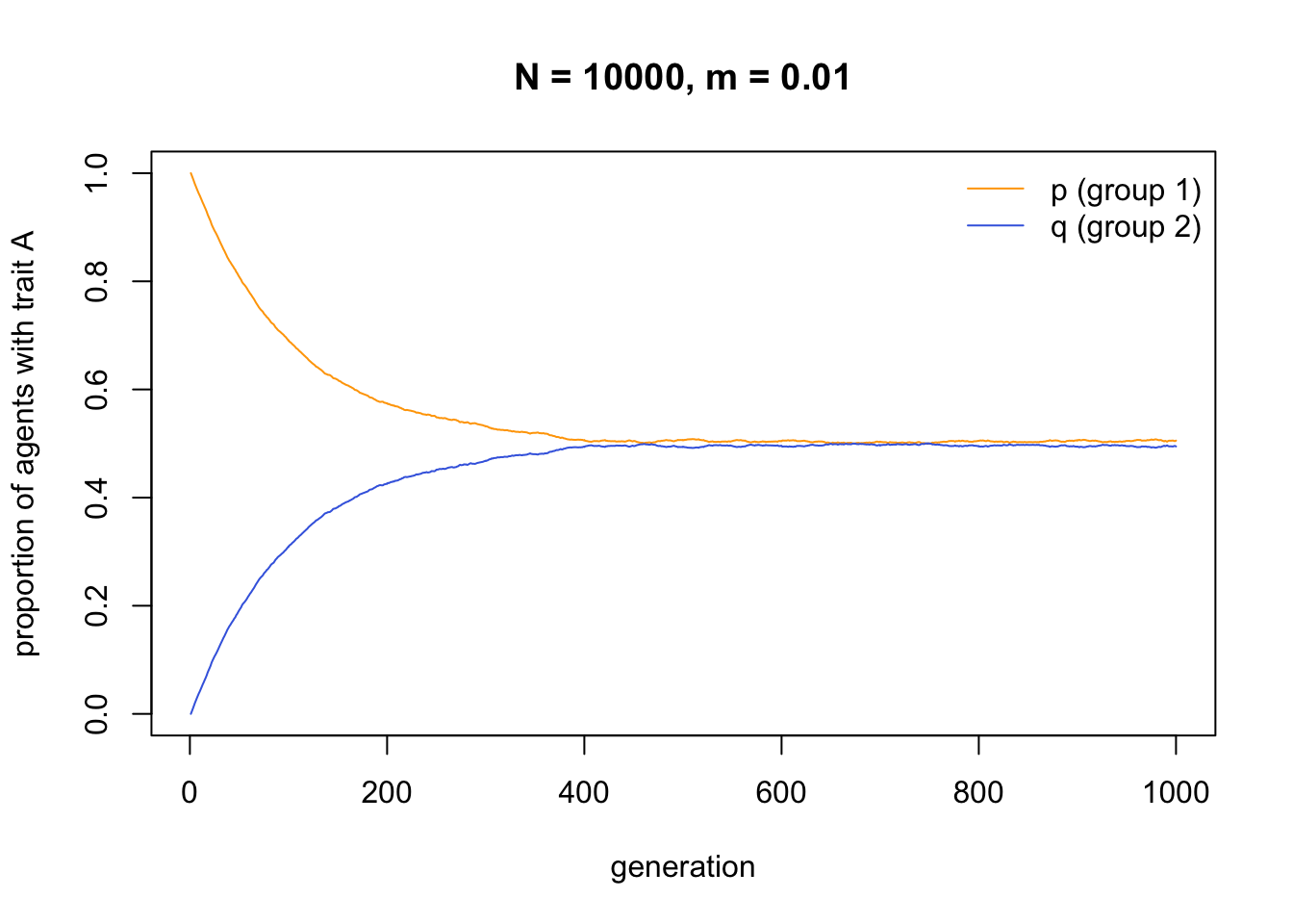
Migration causes both groups to converge on a 50:50 split of \(A\) and \(B\), i.e. \(p = q = 0.5\). Two groups that are initially entirely different in their cultural traits become identical, barring small random fluctuations. Even very small amounts of migration eventually yield between-group homogeneity:
Changing the starting frequencies reveals that \(p\) and \(q\) do not always converge on 0.5. Rather, they converge on the average initial frequency of \(A\) across both groups (i.e. \((p_0 + q_0) / 2\), which in the case below is 0.3):
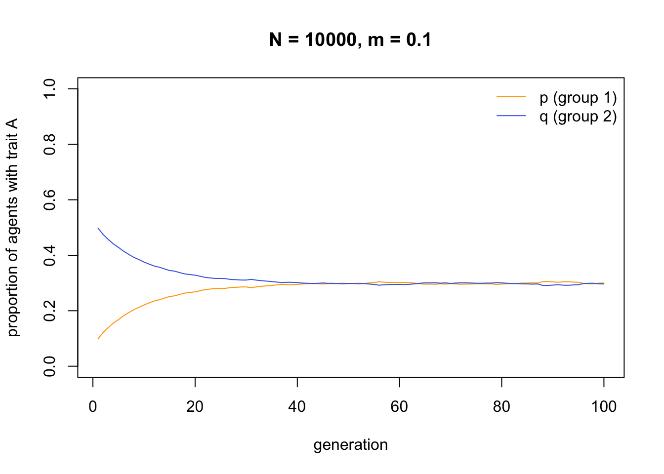
This consequence of migration, to break down between-group differences and make each group identical, is well known from population genetics. In order to maintain between-group variation in the face of even small amounts of migration, we therefore need some additional process.
In genetic evolution one such process is natural selection, if selection favours different alleles in different groups. This might happen, for example, if the groups inhabit different environments in which different traits are optimal. In Model 3 and Model 5 we saw how directly biased transmission and conformist transmission can act as forms of cultural selection. Perhaps, then, these processes can maintain between-group variation in cultural evolution.
The following function adds directly biased transmission using code from the BiasedTransmission function of Model 3. We assume that trait \(A\) is favoured in group 1, and trait \(B\) is favoured in group 2. The parameter \(s\) determines the strength of this biased transmission / cultural selection, which we assume is equal in strength (but opposite in direction) in each group. For simplicity again we’ll omit the multiple runs, hence no \(r_{max}\).
MigrationPlusBiasedTransmission <- function (N, p_0, q_0, m, s, t_max) {

  # create output dataframe to hold t_max values of p and q
  output <- data.frame(p = rep(NA, t_max), q = rep(NA, t_max))

  # create first generation of group 1
  agent1 <- data.frame(trait = sample(c("A","B"), N, replace = TRUE,
                       prob = c(p_0,1-p_0)),
                       group = 1)

  # create first generation of group 2
  agent2 <- data.frame(trait = sample(c("A","B"), N, replace = TRUE,
                       prob = c(q_0,1-q_0)),
                       group = 2)

  # combine agent1 and agent2 into a single agent dataframe
  agent <- rbind(agent1,agent2)

  # store first generation frequencies
  output$p[1] <- sum(agent$trait[agent$group == 1] == "A") / N
  output$q[1] <- sum(agent$trait[agent$group == 2] == "A") / N

  for (t in 2:t_max) {

    # migration:

    # 2N probabilities, one for each agent, to compare against m
    probs <- runif(1:(2*N))

    # with prob m, add an agent's trait to list of migrants
    migrants <- agent$trait[probs < m]

    # put migrants randomly into empty slots
    agent$trait[probs < m] <- sample(migrants, length(migrants))

    # biased transmission:

    # get 2N random numbers, one per agent, each between 0 and 1
    copy <- runif(2*N)

    # group 1 favours A:
    # for each group 1 agent, pick a random agent as demonstrator and store their trait
    demonstrator_trait <- sample(agent$trait[agent$group == 1], N, replace = TRUE)
    # if demonstrator has A and with probability s, copy A from demonstrator
    agent$trait[agent$group == 1 & demonstrator_trait == "A" & copy < s] <- "A"

    # group 2 favours B:
    # for each group 1 agent, pick a random agent as demonstrator and store their trait
    demonstrator_trait <- sample(agent$trait[agent$group == 2], N, replace = TRUE)
    # if demonstrator has B and with probability s, copy B from demonstrator
    agent$trait[agent$group == 2 & demonstrator_trait == "B" & copy < s] <- "B"

    # store frequencies in output slot t
    output$p[t] <- sum(agent$trait[agent$group == 1] == "A") / N
    output$q[t] <- sum(agent$trait[agent$group == 2] == "A") / N

  }

  plot(x = 1:nrow(output), y = output$p,
       type = 'l',
       col = "orange",
       ylab = "proportion of agents with trait A",
       xlab = "generation",
       ylim = c(0,1),
       main = paste("N = ", N, ", m = ", m, ", s = ", s, sep = ""))

  lines(x = 1:nrow(output), y = output$q, col = "royalblue")

  legend("topright",
         legend = c("p (group 1)", "q (group 2)"),
         lty = 1,
         col = c("orange", "royalblue"),
         bty = "n")

  output  # export data from function
}
And we run the function with \(s = 0.1\):
data_model7 <- MigrationPlusBiasedTransmission(N = 10000,
                                               p_0 = 1,
                                               q_0 = 0,
                                               m = 0.1,
                                               s = 0.1,
                                               t_max = 100)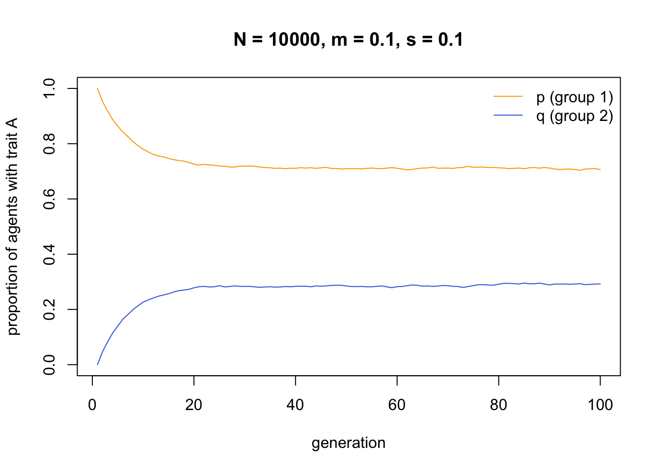
Here we can see how adding cultural selection in the form of directly biased transmission maintains some degree of between-group cultural variation. Group 1 has around 70% \(A\) and 30% \(B\), while group 2 has around 30% \(A\) and 70% \(B\). You can play around with different values of \(s\) and \(m\) to see how the frequencies change in response. When \(s\) is large relative to \(m\), then the groups maintain more distinctive cultural profiles.
Finally, we can see how conformist cultural transmission can also act to maintain between-group cultural variation in the face of migration. The following function integrates the original Migration function above with the ConformistTransmission function from Model 5. Note that conformity operates within each group, on the assumption that individuals are interacting only with other members of their own group, and never with members of the other group.
MigrationPlusConformity <- function (N, p_0, q_0, m, D, t_max) {

  # create output dataframe to hold t_max values of p and q
  output <- data.frame(p = rep(NA, t_max), q = rep(NA, t_max))

  # create first generation of group 1
  agent1 <- data.frame(trait = sample(c("A","B"), N, replace = TRUE,
                       prob = c(p_0,1-p_0)),
                       group = 1)

  # create first generation of group 2
  agent2 <- data.frame(trait = sample(c("A","B"), N, replace = TRUE,
                       prob = c(q_0,1-q_0)),
                       group = 2)

  # combine agent1 and agent2 into a single agent dataframe
  agent <- rbind(agent1,agent2)

  # store first generation frequencies
  output$p[1] <- sum(agent$trait[agent$group == 1] == "A") / N
  output$q[1] <- sum(agent$trait[agent$group == 2] == "A") / N

  for (t in 2:t_max) {

    # migration:

    # 2N probabilities, one for each agent, to compare against m
    probs <- runif(1:(2*N))

    # with prob m, add an agent's trait to list of migrants
    migrants <- agent$trait[probs < m]

    # put migrants randomly into empty slots
    agent$trait[probs < m] <- sample(migrants, length(migrants))

    # conformity in group 1:

    # create dataframe with a set of 3 randomly-picked group 1 demonstrators for each agent
    demonstrators <- data.frame(dem1 = sample(agent$trait[agent$group == 1], N, replace = TRUE),
                                dem2 = sample(agent$trait[agent$group == 1], N, replace = TRUE),
                                dem3 = sample(agent$trait[agent$group == 1], N, replace = TRUE))

    # get the number of As in each 3-dem combo
    numAs <- rowSums(demonstrators == "A")

    agent$trait[agent$group == 1 & numAs == 3] <- "A"  # for dem combos with all As, set to A
    agent$trait[agent$group == 1 & numAs == 0] <- "B"  # for dem combos with no As, set to B

    prob <- runif(N)

    # when A is a majority, 2/3
    agent$trait[agent$group == 1 & numAs == 2 & prob < (2/3 + D/3)] <- "A"
    agent$trait[agent$group == 1 & numAs == 2 & prob >= (2/3 + D/3)] <- "B"

    # when A is a minority, 1/3
    agent$trait[agent$group == 1 & numAs == 1 & prob < (1/3 - D/3)] <- "A"
    agent$trait[agent$group == 1 & numAs == 1 & prob >= (1/3 - D/3)] <- "B"

    # conformity in group 2:

    # create dataframe with a set of 3 randomly-picked group 2 demonstrators for each agent
    demonstrators <- data.frame(dem1 = sample(agent$trait[agent$group == 2], N, replace = TRUE),
                                dem2 = sample(agent$trait[agent$group == 2], N, replace = TRUE),
                                dem3 = sample(agent$trait[agent$group == 2], N, replace = TRUE))

    # get the number of As in each 3-dem combo
    numAs <- rowSums(demonstrators == "A")

    agent$trait[agent$group == 2 & numAs == 3] <- "A"  # for dem combos with all As, set to A
    agent$trait[agent$group == 2 & numAs == 0] <- "B"  # for dem combos with no As, set to B

    prob <- runif(N)

    # when A is a majority, 2/3
    agent$trait[agent$group == 2 & numAs == 2 & prob < (2/3 + D/3)] <- "A"
    agent$trait[agent$group == 2 & numAs == 2 & prob >= (2/3 + D/3)] <- "B"

    # when A is a minority, 1/3
    agent$trait[agent$group == 2 & numAs == 1 & prob < (1/3 - D/3)] <- "A"
    agent$trait[agent$group == 2 & numAs == 1 & prob >= (1/3 - D/3)] <- "B"

    # store frequencies in output slot t
    output$p[t] <- sum(agent$trait[agent$group == 1] == "A") / N
    output$q[t] <- sum(agent$trait[agent$group == 2] == "A") / N

  }

  plot(x = 1:nrow(output), y = output$p,
       type = 'l',
       col = "orange",
       ylab = "proportion of agents with trait A",
       xlab = "generation", ylim = c(0,1),
       main = paste("N = ", N, ", m = ", m, ", D = ", D, sep = ""))

  lines(x = 1:nrow(output), y = output$q, col = "royalblue")

  legend("topright",
         legend = c("p (group 1)", "q (group 2)"),
         lty = 1,
         col = c("orange", "royalblue"),
         bty = "n")

  output  # export data from function
}
With a moderate amount of conformity, \(D = 0.2\), i.e. a 20% chance of adopting the majority trait:
data_model7 <- MigrationPlusConformity(N = 10000,
                                       p_0 = 1,
                                       q_0 = 0,
                                       m = 0.05,
                                       D = 0.2,
                                       t_max = 1000)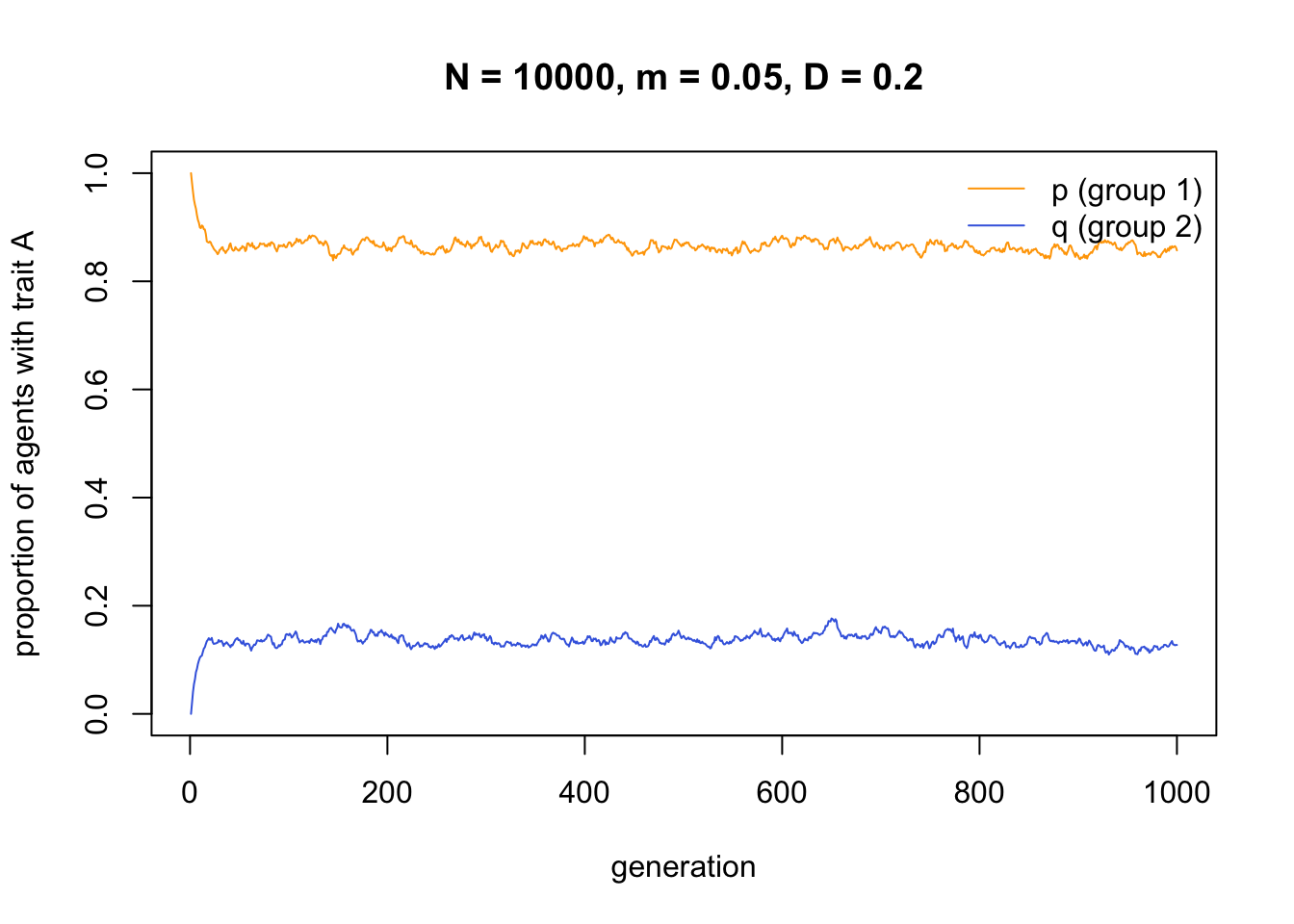
Here again, conformist transmission - a form of cultural selection - maintains between-group cultural variation even in the face of migration. The difference to directly biased transmission is that we do not need to assume different environments or selection pressures in the two groups. Conformity works simply on the basis of the different frequencies of the traits in the different groups.
Summary
Model 7 looked at how migration across group boundaries can break down between-group cultural variation to create a homogenous, undifferentiated mass culture where every group is culturally identical. While globalisation via the mass media or global markets has perhaps been making real-life human societies more similar to one another in recent years, we can still discern culturally distinct societies across the world, marked by traits such as dress, language, religion, psychological characteristics, cuisine and so on. Prior to the invention of mass transit and mass communication, societies would have been even more distinct. Yet migration has been a constant fixture of our species since we dispersed across the world. How then can we reconcile the extensive between-group cultural variation of our species with this frequent migration?
We modelled two potential answers to this question, both forms of cultural selection. Where different traits are favoured in different groups, then directly biased transmission (see Model 3) can maintain between-group cultural variation even in the face of migration. Similarly, conformity (see Model 5) can maintain between-group cultural variation by causing migrants to adopt the majority trait in their new society. The latter works even for neutral, arbitrary traits, which may describe well many real-life group markers. Directly and conformist biased transmission can be seen as mechanisms of acculturation, which describes the cultural change that may occur as a result of migration. Given that psychological processes such as conformity are unique to cultural evolution, this may also be an explanation for why there is a lot more between-group cultural variation in our species than there is between-group genetic variation (for further details and data on migration, conformity and between-group cultural variation, see Henrich & Boyd 1998; Bell et al. 2009; Mesoudi 2018; Deffner et al. 2020).
The major programming innovation in Model 7 was the introduction of two groups of agents. This allows us to simulate migration between groups, as well as processes that are likely to occur predominantly within groups such as conformity. There are many ways of extending Model 7, including adding more groups, adding non-random migration, using measures like \(F_{ST}\) to quantify the amount of between-group cultural variation, making the cultural traits cooperative / non-cooperative rather than neutral, and modelling other processes that might maintain variation such as punishment (see Mesoudi 2018).
Exercises
Try different values of \(m\), \(p_0\) and \(q_0\) in the Migration function to confirm that migration causes groups to converge on the initial mean frequency of trait \(A\) across all groups, i.e. \((p_0+q_0)/2\).
Try different values of \(m\) and \(s\) in MigrationPlusBiasedTransmission, and \(m\) and \(D\) in MigrationPlusConformity, to explore how strong \(s\) and \(D\) need to be relative to \(m\) to prevent population homogenisation.
Add a third group of \(N\) agents. As before, \(m\) is the probability that each agent moves to a random group. Where before there were two groups to randomly select, now there are three. Show that migration still causes convergence on the initial mean frequency of trait \(A\) across all three groups.
Change the function to allow a user-defined number of groups. The function should take the number of groups as a parameter, and create this number of groups on-the-fly. Either allow the user to specify the starting frequencies of \(A\) across all groups (e.g. by having a parameter that can take sets of values such as c(0.3,0.5,0.8,0.9)), or make the starting values random. Show that migration still causes convergence on the initial mean frequency of trait \(A\) across all groups.
Make migration non-random, such that agents are more likely to migrate to groups that have a higher frequency of trait \(A\). How do the dynamics of non-random migration compare to those of the random migration simulated in the original Migration function?
Analytic Appendix
Let’s derive the recursions and equilibrium frequency for the basic migration model, to understand analytically why the frequency of \(A\) in each group converges on the initial average frequency of \(A\) across the two groups.
Recall that the frequency of \(A\) in generation \(t\) in the first group is \(p_t\) and in the second group is \(q_t\). The frequency of \(A\) in the previous generation is denoted \(p_{t-1}\) and \(q_{t-1}\) respectively, and in the first generation it is \(p_0\) and \(q_0\) respectively. Let’s consider group 1 first. We want to write an expression for \(p_t\), in terms of \(p_{t-1}\), the migration rate \(m\), and any other parameter that is necessary.
In generation \(t\), \(1 - m\) individuals in group 1 do not migrate. The frequency of \(A\) amongst these \(1-m\) individuals will therefore be the same as in the previous generation in group 1, i.e. \(p_{t-1}\). This gives an overall frequency for these group 1 non-migrants of \(p_{t-1}(1 - m)\).
The other \(m\) individuals in group 1 are migrants. These migrants are drawn from the entire population, which in this case is groups 1 and 2 combined. The frequency of \(A\) in the entire population is the average frequency of \(A\) across the two groups, which we will denote \(\bar{x}\). The frequency of \(A\) amongst the \(m\) migrants in generation \(t\) in group 1 will therefore be \(\bar{x}m\). What is the value of \(\bar{x}m\)? Because there is no mutation or drift in this model, new \(A\)s never appear, and existing \(A\)s never disappear, when considering the entire population. Hence the total frequency of \(A\) in the entire population will always remain the same, from the first generation to the last. This will be \(\bar{x} = (p_0 + q_0) / 2\), i.e. the average frequency of \(A\) across the two groups in the first generation. This means that \(\bar{x}\) is a constant, i.e. it never changes from one generation to the next.
Putting these together, the frequency of \(A\) in generation \(t\) in group 1, \(p_t\), will be
\[p_t = p_{t-1}(1-m) + \bar{x}m \hspace{30 mm}(7.1)\] Equivalently, the frequency of \(A\) in generation \(t\) in group 2, \(q_t\), will be
\[q_t = q_{t-1}(1-m) + \bar{x}m \hspace{30 mm}(7.2)\] Now we have two recursions, and we can plot them.
MigrationRecursion <- function(m, t_max, p_0, q_0) {

  p <- rep(0,t_max)
  p[1] <- p_0

  q <- rep(0,t_max)
  q[1] <- q_0

  for (i in 2:t_max) {
    x_bar <- (p[i-1] + q[i-1]) / 2

    p[i] <- p[i-1]*(1-m) + x_bar*m

    q[i] <- q[i-1]*(1-m) + x_bar*m
  }

  plot(x = 1:t_max, y = p,
       type = "l",
       ylim = c(0,1),
       ylab = "frequency of A trait",
       xlab = "generation",
       col = "orange",
       main = paste("m = ", m, sep = ""))

  lines(x = 1:t_max, y = q, col = "royalblue")

  abline(h = (p_0 + q_0) / 2, lty = 3)

  legend("topright",
         legend = c("p (group 1)", "q (group 2)"),
         lty = 1,
         col = c("orange", "royalblue"),
         bty = "n")

}

MigrationRecursion(m = 0.1, t_max = 100, p_0 = 1, q_0 = 0)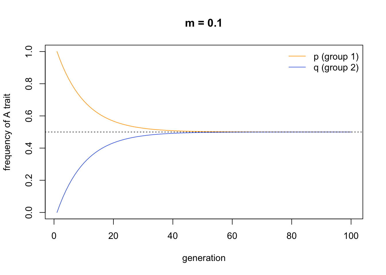
This looks almost identical to the first plot we created above from the simulations. I added a dotted line denoting the initial mean frequency of \(A\) in the entire population, \(\bar{x}\), to verify that the two groups converge on this mean. We can change the starting values to provide a further check:
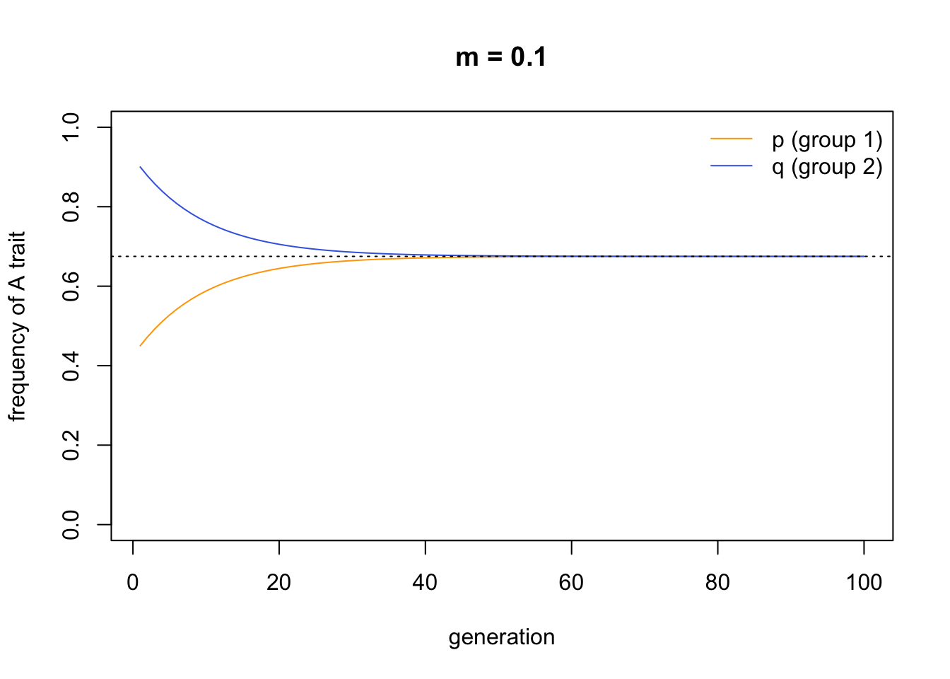
To understand better why this convergence occurs, we need to solve these recursions. Hartl & Clark (1997, p.168) provide a trick for solving such equations, where the recursion can be expressed in the form \(p_t-X = (p_{t-1}-X)Y\), where X and Y are constants. Rearranging this expression gives \(p_t = p_{t-1}Y - XY + X = p_{t-1}Y - X(Y+1)\). This fits equation 7.1 if we say that \(Y = 1 - m\) and \(X = \bar{x}\). Hence we can rewrite equation 7.1 as:
\[p_t - \bar{x} = (p_{t-1} - \bar{x})(1-m) \hspace{30 mm}(7.3)\] Because the relation between \(p_{t-1}\) and \(p_{t-2}\) is the same as that between \(p_t\) and \(p_{t-1}\), all the way back to \(p_0\), the solution to equation 7.3 is
\[p_t - \bar{x} = (p_0 - \bar{x})(1-m)^t \hspace{30 mm}(7.4)\] After many generations, when \(t\) becomes very large, then the last term on the right which is raised to the power of \(t\) will be approximately zero. Even if \(m\) is very small, and \((1 - m)\) is very close to 1, any number less than 1 raised to a large power (i.e. multiplied by itself many times) will be approximately zero. Consequently the whole right hand side of equation 7.4 becomes zero, and \(p_t\) remains the same generation after generation. So we can set the right-hand side of equation 7.4 to zero and rearrange to find this equilibrium value, \(p^*\):
\[p^* = \bar{x} \hspace{30 mm}(7.5)\] And as we noted at the beginning, \(\bar{x} = (p_0 + q_0) / 2\), i.e. the average of the two starting frequencies of \(A\) in the two groups. This is what we found in the agent-based simulations as well as the recursion simulations in this section.
References
Bell, A. V., Richerson, P. J., & McElreath, R. (2009). Culture rather than genes provides greater scope for the evolution of large-scale human prosociality. Proceedings of the National Academy of Sciences, 106(42), 17671-17674.
Deffner, D., Kleinow, V., & McElreath, R. (2020). Dynamic social learning in temporally and spatially variable environments. Royal Society Open Science, 7(12), 200734.
Hartl, D. L., Clark, A. G. (1997). Principles of population genetics. Sunderland, MA: Sinauer associates.
Henrich, J., & Boyd, R. (1998). The evolution of conformist transmission and the emergence of between-group differences. Evolution and Human Behavior, 19(4), 215-241.
Mesoudi, A. (2018). Migration, acculturation, and the maintenance of between-group cultural variation. PLOS ONE, 13(10), e0205573.