Model 1: Unbiased transmission
Introduction
Here we will simulate perhaps the simplest possible case of cultural evolution. We assume \(N\) individuals each of whom possesses one of two cultural traits, denoted \(A\) and \(B\). Each generation, the \(N\) agents are replaced with \(N\) new agents. Each new agent picks a member of the previous generation at random and copies their cultural trait. This is known as unbiased oblique cultural transmission: unbiased because traits are copied entirely at random, and oblique because one generation learns from the previous non-overlapping generation (as opposed to horizontal cultural transmission where individuals copy members of the same generation, and vertical cultural transmission where offspring copy their parents - our model is way too simple to have actual parents and offspring though).
We are interested in tracking the proportion of individuals who possess trait \(A\) over successive generations. We will call this proportion \(p\). We could also track the proportion who possess trait \(B\), but this will always be \(1 - p\) given that everyone who does not possess \(A\) must possess \(B\), so there is really no need. For example, if 70% of the population have trait \(A\), then \(p = 0.7\). The remaining 30% must have trait \(B\), which is a proportion \(1 - p = 1 - 0.7 = 0.3\).
The output of the model will be a plot showing \(p\) over all generations (or timesteps) up to the last generation. Generations are denoted by \(t\), where generation one is \(t = 1\), generation two is \(t = 2\), up to the last generation \(t = t_{max}\). These could correspond to biological generations, but could equally be ‘cultural generations’ (or learning episodes) within the same fixed population, which would be much shorter.
Model 1
First we need to specify the fixed parameters of the model. These are \(N\) (the number of individuals) and \(t_{max}\) (the number of generations). Let’s start with \(N = 100\) and \(t_{max} = 200\).
Run this code snippet in RStudio using the green ‘play’ triangle in the top right of the snippet. If you have the Environment pane visible on the right, you should be able to see \(N\) and \(t_{max}\) appear, with their assigned values. The Environment pane is useful for keeping track of active variables and their current values.
Now we need to create our agents. These will be stored in a dataframe, a commonly-used data format in R. The only information we need to keep about our agents is their cultural trait (\(A\) or \(B\)). Hence we need a dataframe that is \(N\) rows long, with a single column for the trait. We’ll call this dataframe agent. Initially, we will give each agent either an \(A\) or \(B\) at random, using the sample command.
Here, trait specifies the name of the sole variable/column in the agent dataframe. This is filled using sample. The first part of the sample command lists the elements to pick at random, in our case, the traits \(A\) and \(B\). The second part gives the number of times to pick, in our case \(N\) times, once for each agent. The final part says to replace or reuse the elements after they’ve been picked. Otherwise, there would only be one copy of \(A\) and one copy of \(B\), so we could only give two agents traits before running out.
We can see the first few lines of agent using the head command, to check it worked:
##   trait
## 1     A
## 2     A
## 3     A
## 4     B
## 5     A
## 6     A
As expected, there is a single column called trait containing \(A\)s and \(B\)s. Note that head only shows the first 6 rows for brevity; the other 94 are not shown. The numbers on the left are automatically generated in a dataframe as row labels, but in our case we can think of them as the agents’ id numbers (agent 1, agent 2,…, agent 100).
A specific agent’s trait can be retrieved using standard dataframe indexing. For example, agent 4’s trait can be retrieved using:
## [1] "B"This should match the fourth row in the head output above.
We also need a dataframe to track the trait frequency \(p\) in each generation. This will have a single column with \(t_{max}\) rows, one for each generation. We’ll call this dataframe output, because it is the output of the model. At this stage we don’t know what \(p\) will be in each generation, so for now let’s fill the output dataframe with lots of NAs, which is R’s symbol for Not Available, or missing value. We can use the rep (repeat) command to repeat NA \(t_{max}\) times.
Here, \(p\) is the name of the sole variable/column in the output dataframe, and it’s filled entirely with NAs. We’re using NA rather than, say, zero, because zero could be misinterpreted as \(p = 0\), which would mean that all agents have trait \(B\). This would be misleading, because at the moment we haven’t yet calculated \(p\), so it’s non-existent, rather than zero.
We can, however, fill in the first value of \(p\) for our already-created first generation of agents, held in agent. The command below sums the number of \(A\)s in agent and divides by \(N\) to get a proportion out of 1 rather than an absolute number. It then puts this proportion in the first slot of \(p\) in output, the one for the first generation, \(t = 1\). We can again use head to check it worked.
##     p
## 1 0.6
## 2  NA
## 3  NA
## 4  NA
## 5  NA
## 6  NA
This first \(p\) value should be approximately 0.5: maybe not exactly, because we have a finite and relatively small population size. Analogously, flipping a coin 100 times will not always give exactly 50 heads and 50 tails. Sometimes we would get 51 heads, sometimes 52 heads, sometimes 48. Similarly, sometimes we will have 51 \(A\)s, sometimes 48, etc.
Now we need to iterate our population over \(t_{max}\) generations. In each generation, we need to:
copy the current agents to a separate dataframe called previous_agent to use as demonstrators for the new agents; this allows us to implement oblique transmission with its non-overlapping generations, rather than mixing up the generations and getting in a muddle
create a new generation of agents, each of whose trait is picked at random from the previous_agent dataframe
calculate \(p\) for this new generation and store it in the appropriate slot in output
To iterate, we’ll use a for-loop, using \(t\) to track the generation. We’ve already done generation 1 so we’ll start at generation 2. The random picking of models is done with sample again, but this time picking from the traits held in previous_agent. Note that I’ve added comments briefly explaining what each line does. This is perhaps superfluous in a tutorial like this, but it’s always good practice. Code often gets cut-and-pasted into other places and loses its context. Explaining what each line does lets other people - and a future, forgetful you - know what’s going on.
for (t in 2:t_max) {

  # copy agent dataframe to previous_agent dataframe
  previous_agent <- agent

  # randomly copy from previous generation's agents
  agent <- data.frame(trait = sample(previous_agent$trait, N, replace = TRUE))

  # get p and put it into the output slot for this generation t
  output$p[t] <- sum(agent$trait == "A") / N

}
Now we should have 200 values of \(p\) stored in output, one for each generation. Let’s plot them.
plot(output$p,
     type = 'l',
     ylab = "p, proportion of agents with trait A",
     xlab = "generation",
     ylim = c(0,1),
     main = paste("N =", N))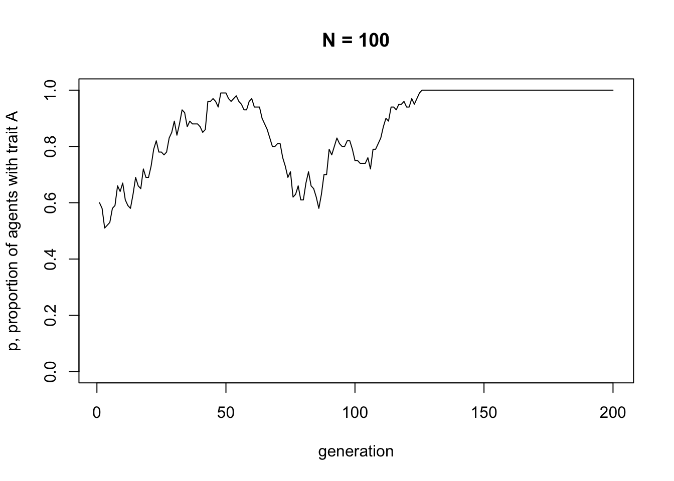
Note the title of the graph, which gives the value of \(N\) for this simulation. It’s easy to create plots and forget what the parameters were. It’s therefore a good idea to include it somewhere on the graph. There’s no need to include our other parameter, \(t_{max}\), because that can be seen from the x-axis scale.
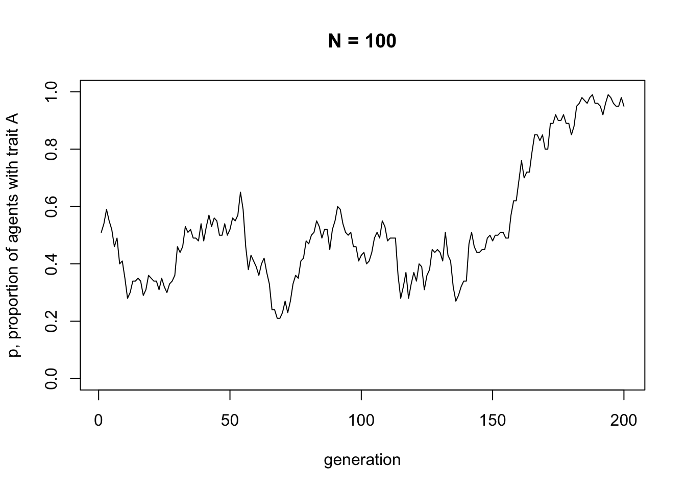
Unbiased transmission, or random copying, is by definition random, so different runs of this simulation will generate different plots. If you rerun all the code you’ll get something different again. It probably starts off hovering around 0.5, the approximate starting value of \(p\), and might go to 0 or 1 at some point. At \(p = 0\) there are no \(A\)s and every agent possesses \(B\). At \(p = 1\) there are no \(B\)s and every agent possesses \(A\). This is a typical feature of cultural drift, analogous to genetic drift: in small populations, with no selection or other directional processes operating, traits can be lost purely by chance.
Ideally we would like to repeat the simulation to explore this idea in more detail, perhaps changing some of the parameters. For example, if we increase \(N\), are we more or less likely to lose one of the traits? With our code scattered about in chunks, it is hard to quickly repeat the simulation. Instead we can wrap it all up in a function, like so:
UnbiasedTransmission <- function (N, t_max) {

  agent <- data.frame(trait = sample(c("A","B"), N, replace = TRUE))

  output <- data.frame(p = rep(NA, t_max))

  output$p[1] <- sum(agent$trait == "A") / N

  for (t in 2:t_max) {

    # copy agent to previous_agent dataframe
    previous_agent <- agent

    # randomly copy from previous generation
    agent <- data.frame(trait = sample(previous_agent$trait, N, replace = TRUE))

    # get p and put it into output slot for this generation t
    output$p[t] <- sum(agent$trait == "A") / N

  }

  plot(output$p,
       type = 'l',
       ylab = "p, proportion of agents with trait A",
       xlab = "generation",
       ylim = c(0,1),
       main = paste("N =", N))

}
This is just all of the code snippets that we already ran above, but all within a function with parameters \(N\) and \(t_{max}\) as arguments to the function. Nothing will happen when you run the above code, because all you’ve done is define the function, not actually run it. The point is that we can now call the function in one go, easily changing the values of \(N\) and \(t_{max}\). Let’s try first with the same values of \(N\) and \(t_{max}\) as before, to check it works. You can re-run the code below several times, to see different dynamics. It should be different every time.
Now let’s try changing the parameters. The following code re-runs the simulation with a much larger \(N\).
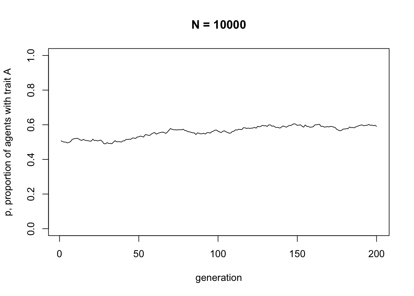
You should see much less fluctuation. Rarely in a population of \(N = 10000\) will either trait go to fixation.
Wrapping a simulation in a function like this is good because we can easily re-run it with just a single command. However, it’s a bit laborious to manually re-run it. Say we wanted to re-run the simulation 10 times with the same parameter values to see how many times \(A\) goes to fixation, and how many times \(B\) goes to fixation. Currently, we’d have to manually run the UnbiasedTransmission function 10 times and record somewhere else what happened in each run. It would be better to automatically re-run the simulation several times and plot each run as a separate line on the same plot. We could also add a line showing the mean value of \(p\) across all runs.
Let’s use a new parameter \(r_{max}\) to specify the number of independent runs, and use another for-loop to cycle over the \(r_{max}\) runs. We also need to expand the number of columns in the output dataframe, because we need one column of \(p\) values for each of the runs. Let’s rewrite the UnbiasedTransmission function to handle multiple runs.
UnbiasedTransmission <- function (N, t_max, r_max) {

  # create a matrix with t_max rows and r_max columns, fill with NAs, convert to dataframe
  output <- as.data.frame(matrix(NA, t_max, r_max))

  # purely cosmetic: rename the columns with run1, run2 etc.
  names(output) <- paste("run", 1:r_max, sep="")

  for (r in 1:r_max) {

    # create first generation
    agent <- data.frame(trait = sample(c("A","B"), N, replace = TRUE))

    # add first generation's p to first row of column r
    output[1,r] <- sum(agent$trait == "A") / N

    for (t in 2:t_max) {

      # copy agent to previous_agent dataframe
      previous_agent <- agent

      # randomly copy from previous generation
      agent <- data.frame(trait = sample(previous_agent$trait, N, replace = TRUE))

      # get p and put it into output slot for this generation t and run r
      output[t,r] <- sum(agent$trait == "A") / N

    }

  }

  # first plot a thick line for the mean p
  plot(rowMeans(output),
       type = 'l',
       ylab = "p, proportion of agents with trait A",
       xlab = "generation",
       ylim = c(0,1),
       lwd = 3,
       main = paste("N =", N))

  for (r in 1:r_max) {

    # add lines for each run, up to r_max
    lines(output[,r], type = 'l')

  }

  output  # export data from function
}
There are a few changes here. First, we created output initially as a matrix, and then immediately converted it into a dataframe. This seems weird, but is just because it is easier to create a multi-row data structure using the matrix command than the dataframe command. The next command is purely cosmetic, and re-names the columns of outcome as run1, run2 etc.
Then we set up our \(r\) loop, which executes once for each run. The code is mostly the same as before, except that we now use the “[row,column]” notation to put \(p\) into the right place in output. The row is \(t\) as before, and now the column is \(r\). The plot command is also changed to handle multiple runs: first we plot the mean as a thick line, then we add one plotted line for each run.
Finally, the UnbiasedTransmission function now ends with the output dataframe. This means that this dataframe will be exported from the function when it is run. This can be useful for storing data from simulations wrapped in functions, otherwise that data is lost after the function is executed. In the function call below, the raw data from the simulation is put into a dataframe called data_model1, as a record of what happened. Run it now to display the new plot.
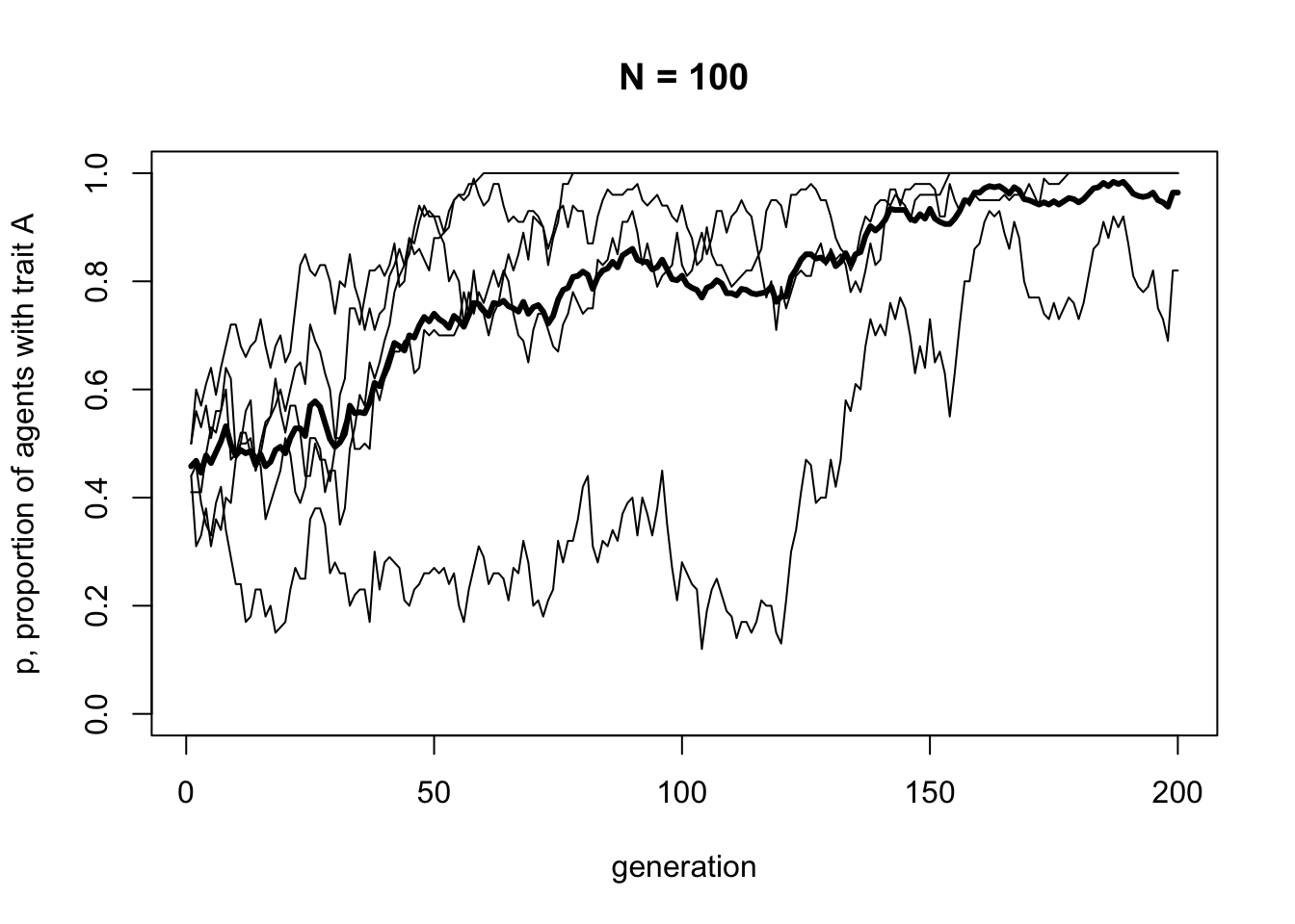
You should be able to see five independent runs of our simulation shown as regular thin lines, along with a thicker line showing the mean of these lines. Some runs have probably gone to 0 or 1, and the mean should be somewhere in between. The data is stored in data_model1, which we can inspect with head:
##   run1 run2 run3 run4 run5
## 1 0.44 0.41 0.50 0.44 0.50
## 2 0.31 0.41 0.60 0.46 0.56
## 3 0.33 0.41 0.57 0.39 0.53
## 4 0.38 0.48 0.61 0.35 0.57
## 5 0.31 0.53 0.64 0.33 0.51
## 6 0.36 0.52 0.59 0.39 0.56
Now let’s run the updated UnbiasedTransmission model with \(N = 10000\), to compare with \(N = 100\).
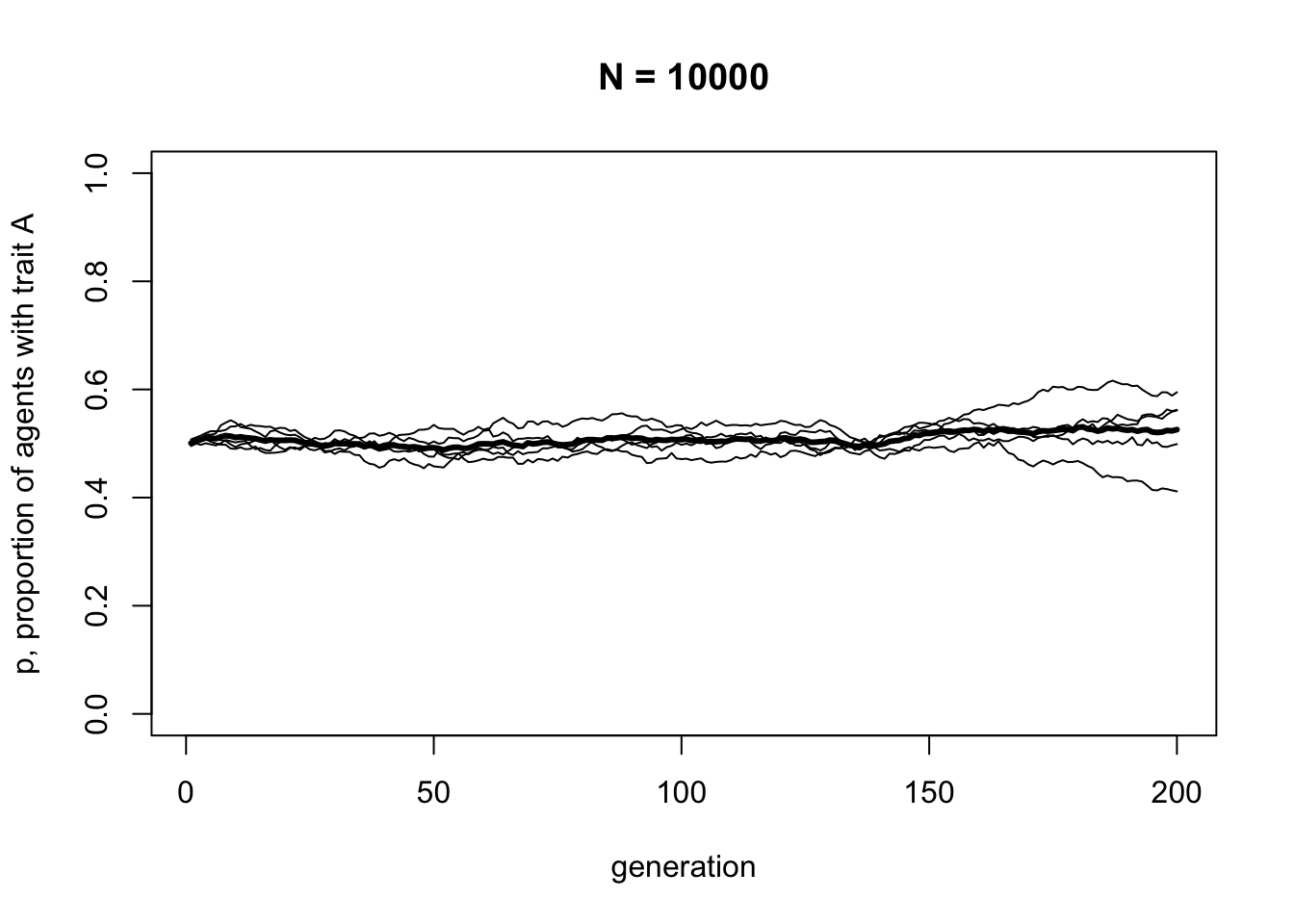
The mean line should be almost exactly at \(p = 0.5\) now, with the five independent runs fairly close to it.
Let’s add one final modification. So far the starting frequencies of \(A\) and \(B\) have been the same, roughly 0.5 each. But what if we were to start at different initial frequencies of \(A\) and \(B\)? Say, \(p = 0.2\) or \(p = 0.9\)? Would unbiased transmission keep \(p\) at these initial values, or would it go to \(p = 0.5\) as we have found so far?
To find out, we can add another parameter, \(p_0\), which specifies the initial probability of drawing an \(A\) rather than a \(B\) in the first generation. Previously this was always \(p_0 = 0.5\), but in the new function below we add it to the sample function to weight the initial allocation of traits in \(t = 1\).
UnbiasedTransmission <- function (N, p_0, t_max, r_max) {

  # create a matrix with t_max rows and r_max columns, fill with NAs, convert to dataframe
  output <- as.data.frame(matrix(NA,t_max,r_max))

  # purely cosmetic: rename the columns with run1, run2 etc.
  names(output) <- paste("run", 1:r_max, sep="")

  for (r in 1:r_max) {

    # create first generation
    agent <- data.frame(trait = sample(c("A","B"), N, replace = TRUE,
                                       prob = c(p_0,1-p_0)))

    # add first generation's p to first row of column r
    output[1,r] <- sum(agent$trait == "A") / N

    for (t in 2:t_max) {

      # copy agent to previous_agent dataframe
      previous_agent <- agent

      # randomly copy from previous generation
      agent <- data.frame(trait = sample(previous_agent$trait, N, replace = TRUE))

      # get p and put it into output slot for this generation t and run r
      output[t,r] <- sum(agent$trait == "A") / N

    }

  }

  # first plot a thick line for the mean p
  plot(rowMeans(output),
       type = 'l',
       ylab = "p, proportion of agents with trait A",
       xlab = "generation",
       ylim = c(0,1),
       lwd = 3,
       main = paste("N =", N))

  for (r in 1:r_max) {

    # add lines for each run, up to r_max
    lines(output[,r], type = 'l')

  }

  output  # export data from function
}
The only change here is the addition of \(p_0\) as a definable parameter for the function, and the prob argument in the sample command. The prob argument gives the probability of picking each option, in our case \(A\) and \(B\), in the first generation. The probability of \(A\) is now \(p_0\), and the probability of \(B\) is now \(1 - p_0\). Let’s see what happens with a different value of \(p_0\).
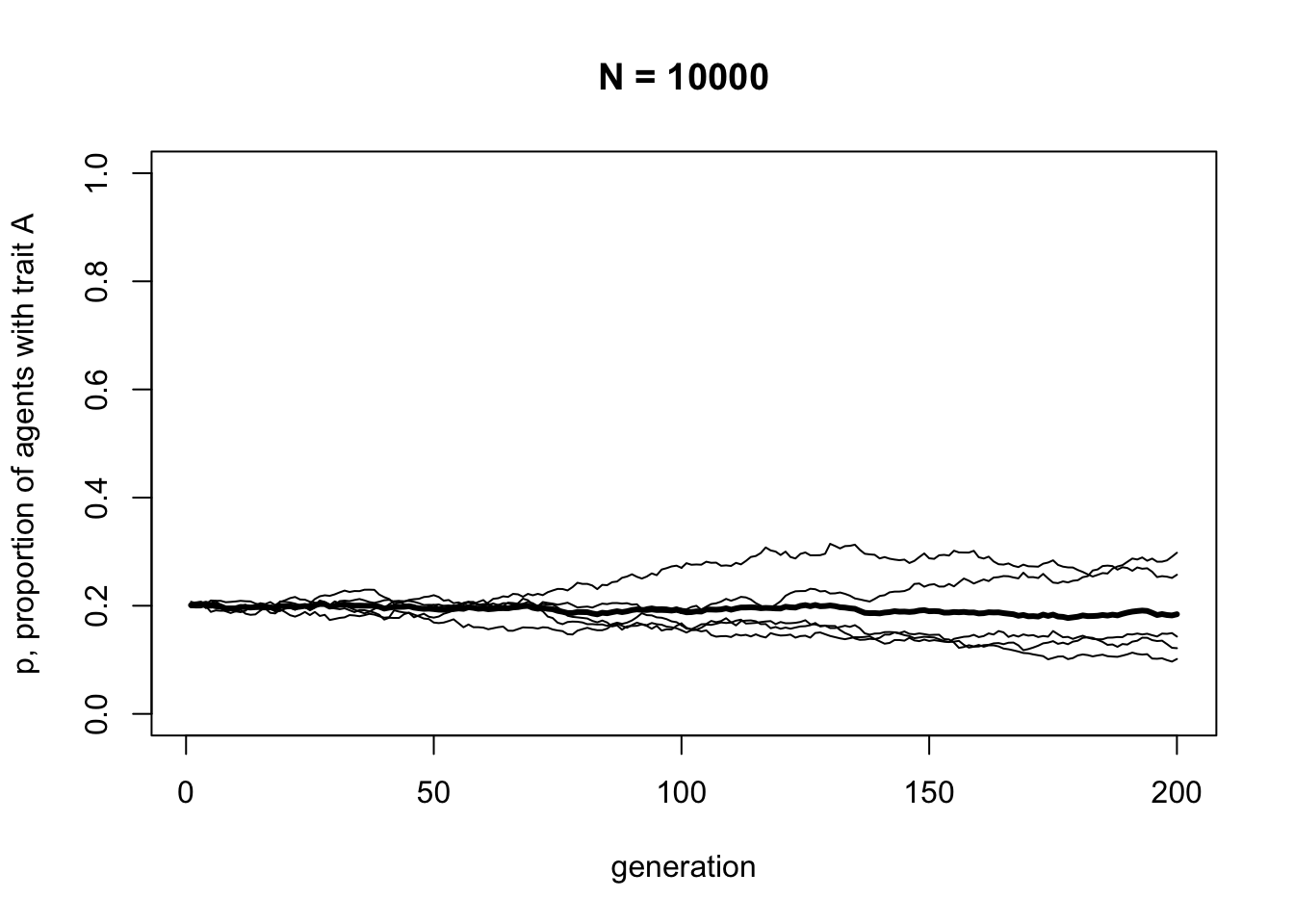
With \(p_0 = 0.2\), trait frequencies stay at \(p = 0.2\). Unbiased transmission is truly non-directional: it maintains trait frequencies at whatever they were in the previous generation, barring random fluctuations caused by small population sizes.
A final useful skill is to be able to export the plot we created to an external image file. This file can then be inserted into other documents, e.g. as a figure in a manuscript. This is done in the code below by wrapping the UnbiasedTransmission function (or any function that outputs a plot) within two commands. First, the png command specifies the file format (you can also use bmp, jpeg or tiff), and takes arguments that set the file name, height and width, units of the height and width (“cm”, “mm”, “in” or “px”), and resolution (in ppi, pixels per inch). Then after the plot is created using UnbiasedTransmission, the dev.off() command tells R that we are done plotting and can export the file. It’s wrapped in invisible just to hide the text output in this Rmd file.
Note that this code puts the plot file into the current working directory. To set the working directory to the same place as this Rmd file, use the menu command Session->Set Working Directory->To Source File Location before running the code below. Otherwise, use the command setwd to set the working directory to somewhere else, or add a full path to the file argument below, within the quote marks where the file name is given.
png(file = "unbiased_transmission.png",
height = 10,
width = 12,
units = "cm" ,
res = 300)
data_model1 <- UnbiasedTransmission(N = 10000,
                                    p_0 = 0.2,
                                    t_max = 200,
                                    r_max = 5)
invisible(dev.off())Summary
Even this extremely simple model provides some valuable insights. First, unbiased transmission does not in itself change trait frequencies. As long as populations are large, trait frequencies remain the same.
Second, the smaller the population size, the more likely traits are to be lost by chance. This is a basic insight from population genetics, known there as genetic drift, but it can also be applied to cultural evolution. More advanced models of cultural drift (sometimes called ‘random copying’) can be found in Cavalli-Sforza & Feldman (1981) and Bentley et al. (2004), with the latter showing that various real-world cultural traits exhibit dynamics consistent with this kind of process, including baby names, dog breeds and archaeological pottery types.
Furthermore, generating expectations about cultural change under simple assumptions like random cultural drift can be useful for detecting non-random patterns like selection. If we don’t have a baseline, we won’t know selection or other directional processes when we see them.
In Model 1 we have introduced several programming techniques that will be useful in later models. We’ve seen how to use dataframes to hold characteristics of agents, how to use loops to cycle through generations and simulation runs, how to use sample to pick randomly from sets of elements, how to wrap simulations in functions to easily re-run them with different parameter values, how to plot the results of simulations, how to store the output of the simulation in a dataframe that persists after the simulation function is run, and how to export a plot to an external image file.
Exercises
Try different values of \(p_0\) with large \(N\) to confirm that unbiased transmission does not change the frequency of \(p\), irrespective of the starting value \(p_0\).
Re-run the UnbiasedTransmission model to find the approximate value of \(N\) at which one of the traits rarely, if ever, goes to fixation after a reasonably large number of timesteps (‘fixation’ means that \(p\) goes to either zero or one and stays there).
Modify the UnbiasedTransmission function to record and output the number of timesteps it takes for a run to go to fixation, i.e. \(p\) goes to zero or one. If a run does not go to fixation after a sufficiently large number of timesteps, record this as NA. Make a plot of time to fixation against population size \(N\). Before creating the plot, what do you think the plot will look like?
Analytical Appendix
If \(p\) is the frequency of \(A\) in one generation, we are interested in calculating \(p'\), the frequency of \(A\) in the next generation under the assumption of unbiased transmission. Each new individual in the next generation picks a demonstrator at random from amongst the previous generation. The demonstrator will have \(A\) with probability \(p\). The frequency of \(A\) in the next generation, then, is simply the frequency of \(A\) in the previous generation:
\[p' = p \hspace{30 mm}(1.1)\]
Equation 1.1 simply says that under unbiased transmission there is no change in \(p\) over time. If, as we assumed above, the initial value of \(p\) in a particular population is \(p_0\), then the equilibrium value of \(p\), \(p^*\), at which there is no change in \(p\) over time, is just \(p_0\).
We can plot this recursion, to recreate the final simulation plot above:
p_0 <- 0.2
t_max <- 200

p <- rep(NA, t_max)
p[1] <- p_0

for (i in 2:t_max) {
  p[i] <- p[i-1]
}

plot(p,
     type = 'l',
     ylab = "p, proportion of agents with trait A",
     xlab = "generation",
     ylim = c(0,1),
     lwd = 3)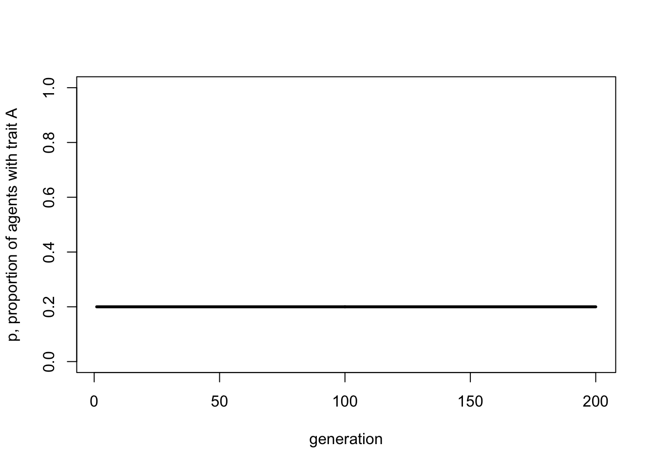
Don’t worry, it gets more complicated than this in later chapters. The key point here is that analytical or deterministic models like these assume infinite populations - note there is no \(N\) in the above recursion - and no stochasticity. Simulations with very large populations should give the same results as analytical models. Basically, the closer we can get in stochastic models to the assumption of infinite populations, the closer the match to infinite-population deterministic models. Deterministic models give the ideal case; stochastic models permit more realistic dynamics based on finite populations.
More generally, creating deterministic recursion-based models can be a good way of verifying simulation models, and vice versa. If the same dynamics occur in both agent-based and recursion-based models, then we can be more confident that those dynamics are genuine and not the result of a programming error or mathematical mistake.
References
Bentley, R. A., Hahn, M. W., & Shennan, S. J. (2004). Random drift and culture change. Proceedings of the Royal Society of London B, 271(1547), 1443-1450.
Cavalli-Sforza, L. L., & Feldman, M. W. (1981). Cultural transmission and evolution: a quantitative approach. Princeton University Press.