Model 6: Vertical and horizontal cultural transmission
Introduction
One obvious difference between cultural and genetic evolution is in their pathways of transmission. In genetic evolution - in humans at least - we get our genes exclusively from our two biological parents. In cultural evolution, we get cultural traits (ideas, attitudes, skills, languages etc.) from a wide array of sources, not just our biological parents but also other relatives, biologically unrelated teachers and peers, or complete strangers via books or the internet.
All of the models we have made so far assume oblique cultural transmission, such that agents learn from one or more members of the previous generation. In Model 6 we will consider vertical cultural transmission, in which agents learn from two parents, and horizontal cultural transmission, where agents learn from members of the same generation.
The models are still extremely simple, with no actual biological reproduction or proper family lineages. We are also maintaining the non-overlapping generations of prior models, which neatly separates each generation. Real life is more messy, with overlapping generations that blur distinctions between, say, oblique and horizontal transmission. But as we have seen, models are useful because of, not despite, their simplicity. In this case, we consider three interesting features of vertical and horizontal transmission. First, the case of assortative cultural mating, where one’s parents are more similar in cultural traits than two randomly chosen members of the population. Second, the case where biases in vertical and horizontal transmission act in opposite directions. Third, we examine the claim that cultural evolution is faster than genetic evolution because it features horizontal transmission.
All of these pathways of transmission were modelled in depth by Cavalli-Sforza & Feldman (1981), and the simulation models here follow their general form.
Model 6a: Vertical cultural transmission
Following the same approach as we did for conformity in Model 4, we can make a table specifying the outcome of vertical cultural transmission for an offspring’s cultural traits given its two parents’ cultural traits. As before, we will use two discrete traits \(A\) and \(B\), with the frequency of \(A\) being \(p\) and of \(B\) being \(1 - p\).
| Mother’s trait | Father’s trait | Probability of child adopting \(A\) |
|---|---|---|
| \(A\) | \(A\) | 1 |
| \(A\) | \(B\) | \(1/2 + s_v/2\) |
| \(B\) | \(A\) | \(1/2 + s_v/2\) |
| \(B\) | \(B\) | 0 |
This table assumes that if both parents have the same trait, then the child inherits that trait with 100% certainty. If parents have different traits, then the child has a 50% chance of inheriting either one, plus an additional chance \(s_v / 2\). This is similar to the conformity parameter \(D\) in giving an adoption boost to a trait, except that now trait \(A\) is always getting a boost, irrespective of which parent has \(A\).
Consequently, \(s_v\) can be seen as a form of directly biased transmission or cultural selection, similar to that explored in Model 3: it gives the probability of preferentially adopting trait \(A\) above that expected under unbiased cultural transmission. It ranges from zero (unbiased transmission) to one (fully biased transmission, where \(A\) is always adopted if either parent has it). It can also be negative (up to -1), in which case trait \(B\) is favoured over \(A\).
The following function takes the structure of ConformistTransmission from Model 5, replacing the three randomly-chosen demonstrators with two randomly-chosen parents, and setting the offspring traits as per the table above.
VerticalTransmission <- function (N, p_0, s_v, t_max, r_max) {

  # create matrix with t_max rows and r_max columns, fill with NAs, convert to dataframe
  output <- as.data.frame(matrix(NA,t_max,r_max))

  # purely cosmetic: rename the columns with run1, run2 etc.
  names(output) <- paste("run", 1:r_max, sep="")

  for (r in 1:r_max) {

    # create first generation
    agent <- data.frame(trait = sample(c("A","B"), N, replace = TRUE,
                        prob = c(p_0,1-p_0)))

    # add first generation's p to first row of column r
    output[1,r] <- sum(agent$trait == "A") / N

    for (t in 2:t_max) {

      # create dataframe with a set of 2 randomly-picked parents for each agent
      parents <- data.frame(mother = sample(agent$trait, N, replace = TRUE),
                            father = sample(agent$trait, N, replace = TRUE))

      prob <- runif(N)

      # if both parents have A, child has A
      agent$trait[parents$mother == "A" & parents$father == "A"] <- "A"

      # if both parents have B, child has B
      agent$trait[parents$mother == "B" & parents$father == "B"] <- "B"

      # if mother has A and father has B, child has A with prob (1/2 + s_v/2), otherwise B
      agent$trait[parents$mother == "A" & parents$father == "B" &
                  prob < (1/2 + s_v/2)] <- "A"
      agent$trait[parents$mother == "A" & parents$father == "B" &
                  prob >= (1/2 + s_v/2)] <- "B"

      # if mother has B and father has A, child has A with prob (1/2 + s_v/2), otherwise B
      agent$trait[parents$mother == "B" & parents$father == "A" &
                  prob < (1/2 + s_v/2)] <- "A"
      agent$trait[parents$mother == "B" & parents$father == "A" &
                  prob >= (1/2 + s_v/2)] <- "B"

      # get p and put it into output slot for this generation t and run r
      output[t,r] <- sum(agent$trait == "A") / N

    }

  }

  # first plot a thick line for the mean p
  plot(rowMeans(output),
       type = 'l',
       ylab = "p, proportion of agents with trait A",
       xlab = "generation",
       ylim = c(0,1),
       lwd = 3,
       main = paste("N = ", N, ", s_v = ", s_v, sep = ""))

  for (r in 1:r_max) {

    # add lines for each run, up to r_max
    lines(output[,r], type = 'l')

  }

  output  # export data from function
}
First we can check that when \(s_v = 0\), we do indeed see unbiased transmission:
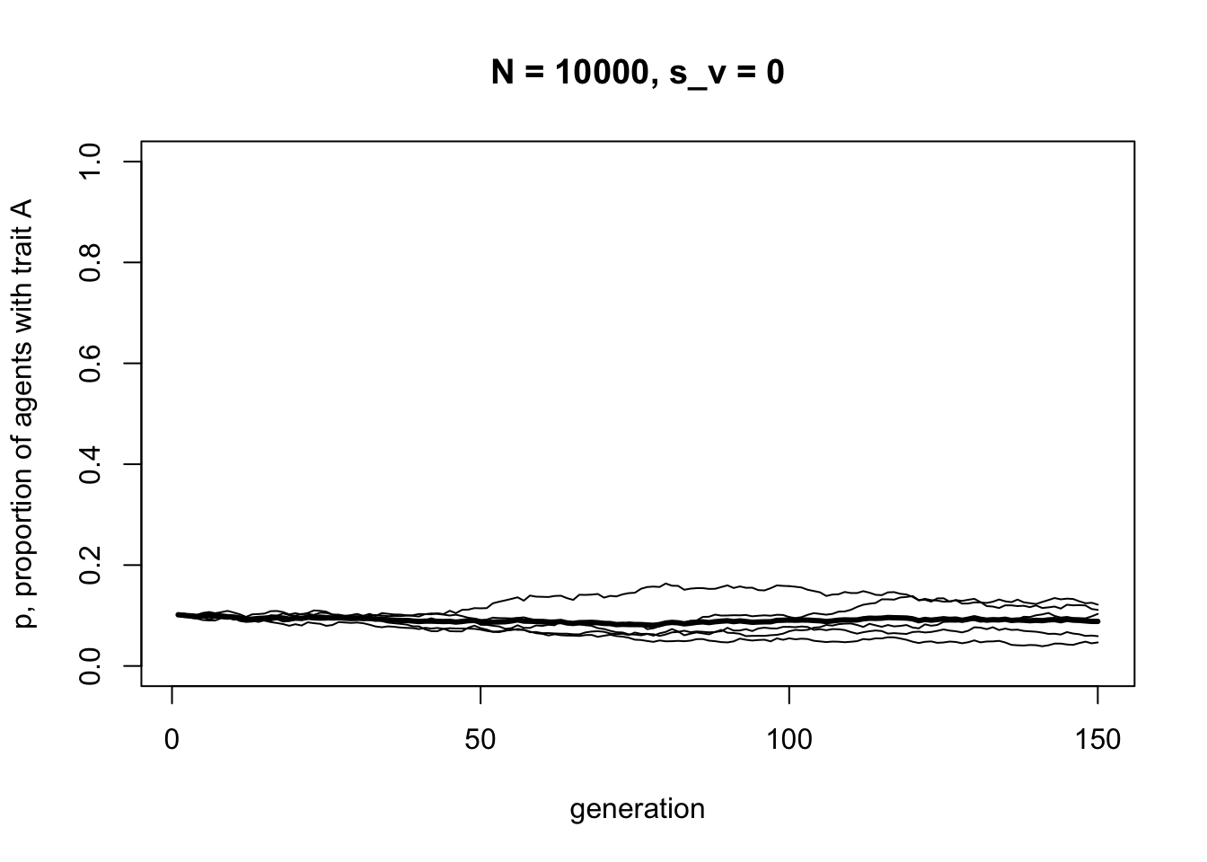
As in previous models, unbiased transmission results in no change in trait frequencies except random fluctuation due to chance. Now we can add selection:
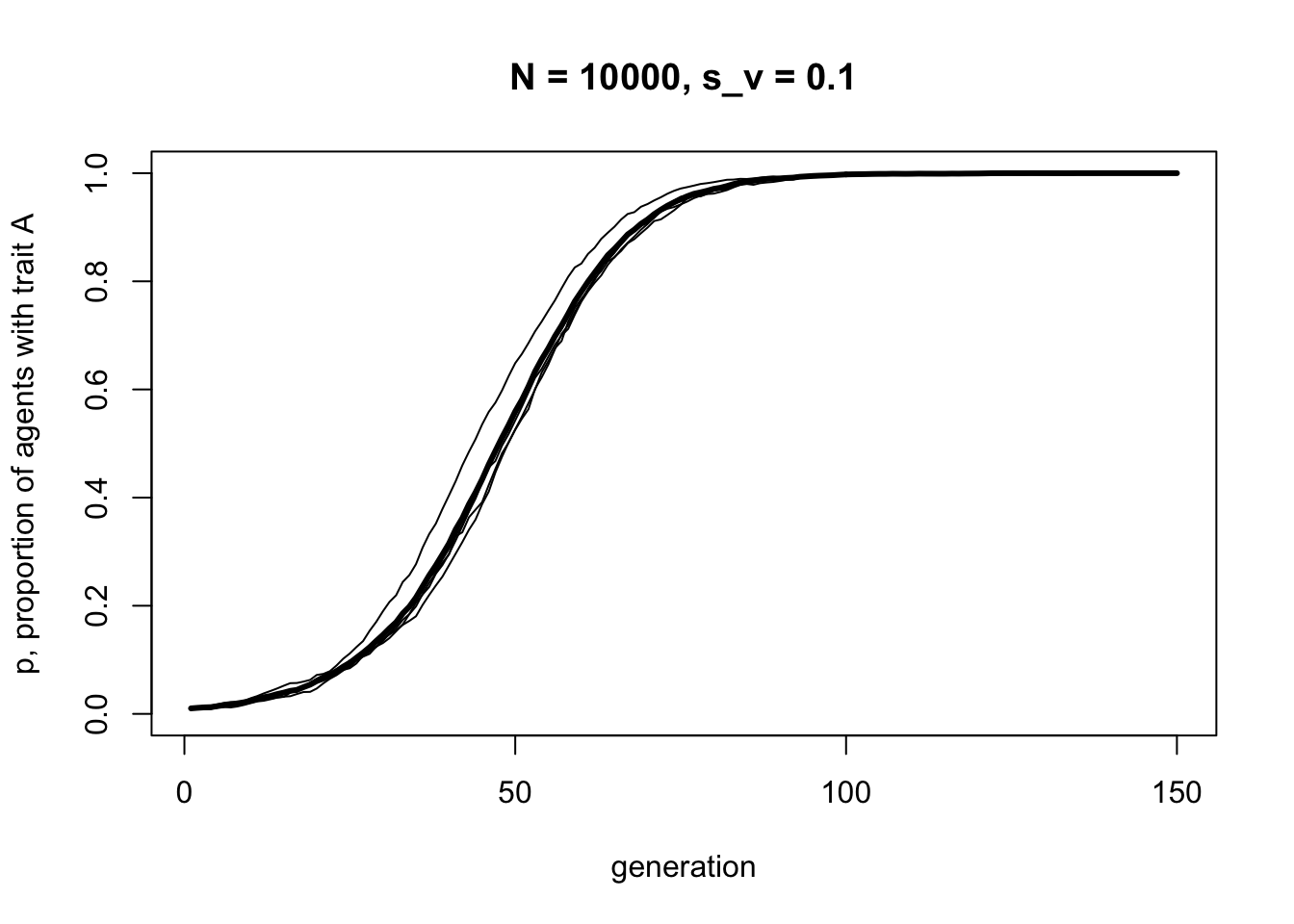
This looks a lot like the s-shaped curve we found in Model 3 for \(s = 0.1\). We have recapitulated unbiased transmission from Model 2 combined with biased transmission from Model 3, but assuming vertical cultural transmission from two parents, rather than randomly picking one demonstrator from the previous generation.
Model 6b: Assortative mating
We can use this vertical transmission model to explore what happens when we relax our assumption that parents form entirely at random. In reality, parents may be more culturally similar than average: two conservatives (or two liberals) may be more likely to get together than a conservative and a liberal; two vegans more likely than one vegan and one meat-eater. In evolutionary biology, this is known as assortative mating. For genetic evolution, it is assumed that the mates assort on genetically inherited characteristics. In cultural evolution, the mates assort on culturally inherited characteristics.
We now assume that a fraction \(a\) of matings are assortative, such that they must involve two parents with identical cultural traits, either both \(A\) or both \(B\). A fraction \(1 - a\) of matings are random as before, and can be any combination of traits. The following function implements this.
VerticalAssortative <- function (N, p_0, s_v, a, t_max, r_max) {

  # create matrix with t_max rows and r_max columns, fill with NAs, convert to dataframe
  output <- as.data.frame(matrix(NA,t_max,r_max))

  # purely cosmetic: rename the columns with run1, run2 etc.
  names(output) <- paste("run", 1:r_max, sep="")

  for (r in 1:r_max) {

    # create first generation
    agent <- data.frame(trait = sample(c("A","B"), N, replace = TRUE,
                        prob = c(p_0,1-p_0)))

    # add first generation's p to first row of column r
    output[1,r] <- sum(agent$trait == "A") / N

    for (t in 2:t_max) {

      # 1. assortative mating:

      # create dataframe with a set of 2 parents for each agent
      # mother is picked randomly, father is blank for now
      parents <- data.frame(mother = sample(agent$trait, N, replace = TRUE),
                            father = rep(NA, N))

      # probabilities for a
      prob <- runif(N)

      # with prob a, make father identical
      parents$father[prob < a] <- parents$mother[prob < a]

      # with prob 1-a, pick random trait for father
      parents$father[prob >= a] <- sample(agent$trait,
                                          sum(prob >= a),
                                          replace = TRUE)

      # 2. vertical transmission:

      # new probabilities for s_v
      prob <- runif(N)

      # if both parents have A, child has A
      agent$trait[parents$mother == "A" & parents$father == "A"] <- "A"

      # if both parents have B, child has B
      agent$trait[parents$mother == "B" & parents$father == "B"] <- "B"

      # if mother has A and father has B, child has A with prob (1/2 + s_v/2), otherwise B
      agent$trait[parents$mother == "A" & parents$father == "B" &
                  prob < (1/2 + s_v/2)] <- "A"
      agent$trait[parents$mother == "A" & parents$father == "B" &
                  prob >= (1/2 + s_v/2)] <- "B"

      # if mother has B and father has A, child has A with prob (1/2 + s_v/2), otherwise B
      agent$trait[parents$mother == "B" & parents$father == "A" &
                  prob < (1/2 + s_v/2)] <- "A"
      agent$trait[parents$mother == "B" & parents$father == "A" &
                  prob >= (1/2 + s_v/2)] <- "B"

      # 3. store results:

      # get p and put it into output slot for this generation t and run r
      output[t,r] <- sum(agent$trait == "A") / N

    }

  }

  # first plot a thick line for the mean p
  plot(rowMeans(output),
       type = 'l',
       ylab = "p, proportion of agents with trait A",
       xlab = "generation",
       ylim = c(0,1),
       lwd = 3,
       main = paste("N = ", N, ", s_v = ", s_v, ", a = ", a, sep = ""))

  for (r in 1:r_max) {

    # add lines for each run, up to r_max
    lines(output[,r], type = 'l')

  }

  output  # export data from function
}
Most of VerticalAssortative is the same as VerticalTransmission, except for changes in the way parents are created. Rather than picking all mothers and fathers randomly, we first pick mothers randomly, then with probability \(a\) give the fathers the same cultural trait as the mother. With probability \(1 - a\) we pick traits randomly for fathers, as in VerticalTransmission. The rest is the same, except that we add \(a\) to the figure title.
Let’s first check that when \(a = 0\), i.e. no assortative mating, the output is identical to that with VerticalTransmission above:
data_model6b <- VerticalAssortative(N = 10000,
                                    p_0 = 0.01,
                                    s_v = 0.1,
                                    a = 0,
                                    t_max = 150,
                                    r_max = 5)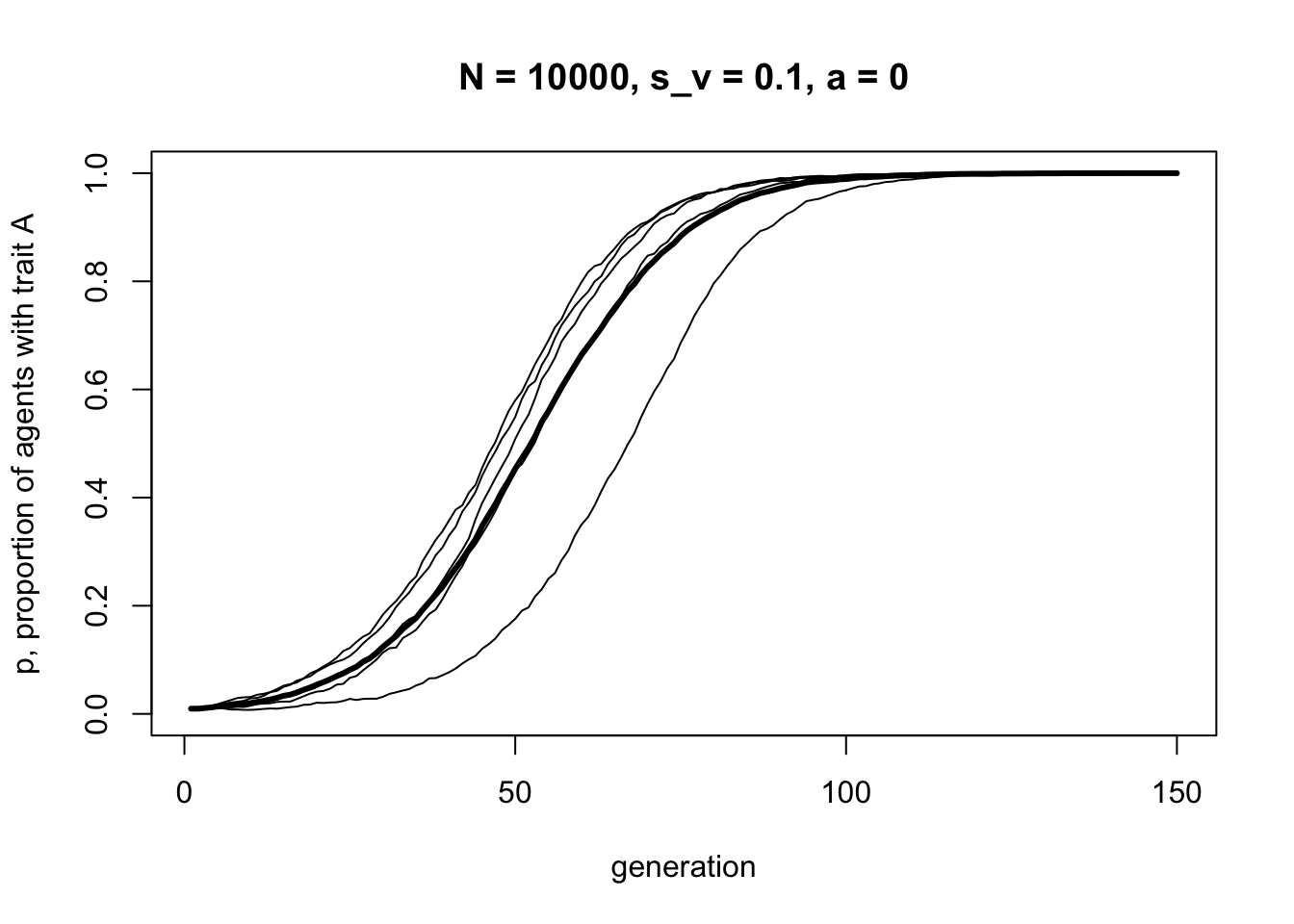
It’s identical to before, with an s-shaped curve indicative of directly biased transmission. Now let’s add some assortative mating, with \(a = 0.4\):
data_model6b <- VerticalAssortative(N = 10000,
                                    p_0 = 0.01,
                                    s_v = 0.1,
                                    a = 0.4,
                                    t_max = 150,
                                    r_max = 5)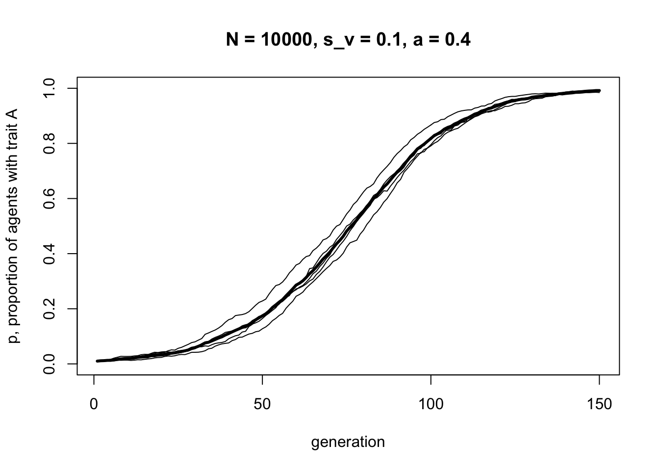
The curve is still s-shaped, but takes longer to reach \(p = 1\). What happens when all mating is assortative, i.e. \(a = 1\)?
data_model6b <- VerticalAssortative(N = 10000,
                                    p_0 = 0.01,
                                    s_v = 0.1,
                                    a = 1,
                                    t_max = 150,
                                    r_max = 5)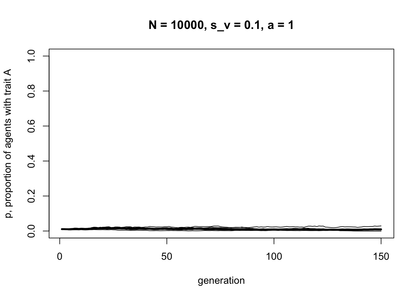
Complete assortative mating results in no cultural change, beyond random fluctuations, even when selection is acting. In general, the more assortative mating there is, the weaker cultural selection will be.
In hindsight this is perhaps obvious. If assortative mating results in parents who have identical cultural traits, and as per the table above identical parents always give rise to identical children, then there will be no change resulting from these matings even when \(s_v > 0\). However, under different assumptions about mating and transmission this may not always be the case. And hindsight does not always match foresight. It’s always good to check and verify even simple predictions and intuitions.
Model 6c: Horizontal cultural transmission
Now we can add horizontal cultural transmission, which involves learning from members of the same generation. We will build this into the VerticalAssortative function above, such that vertical transmission (with assortative mating if \(a > 0\)) occurs first, and then horizontal cultural transmission occurs within the new generation of agents that form after vertical transmission.
There are many ways of implementing horizontal cultural transmission, just like there are many ways of implementing oblique transmission, as covered in other models (e.g. directly biased transmission, conformist biased transmission, blending inheritance). To allow a comparison with vertical transmission, here we will assume directly biased horizontal transmission. We will use a slightly different version of directly biased transmission from Model 3, modified to capture the key advantage of horizontal transmission over vertical transmission: the larger number of potential demonstrators.
Recall that Model 3 involved each agent randomly choosing one member of the previous generation and, if that demonstrator has trait \(A\), then trait \(A\) is adopted with probability \(s\). This reflects a situation where \(A\) is favoured by selection: perhaps \(A\) is a more effective tool, more memorable story, or more easily pronounced word. We are interested in when and how \(A\) spreads when initially rare in the population.
In Model 6c we assume that agents now choose \(n\) members of the same generation, i.e. the set of agents who have already undergone vertical transmission. If at least one of those \(n\) demonstrators has trait \(A\), then the learner adopts trait \(A\) with probability \(s_h\).
This is directly biased transmission, as in Model 3, because \(s_h\) allows agents with \(B\) to switch to \(A\). There is no possibility of agents with \(A\) switching to \(B\). The difference from Model 3 is that now there are \(n\) demonstrators rather than one, and we use the symbol \(s_h\) to distinguish this selection parameter from the one incorporated into vertical transmission, \(s_v\), and the one originally used in Model 3, \(s\).
The following function adds horizontal transmission to VerticalAssortative. We add \(n\) and \(s_h\) to the parameter list, and add some code to implement the horizontal transmission rule.
VerticalHorizontal <- function (N, p_0, s_v, s_h, a, n, t_max, r_max, make_plot = TRUE) {

  # create matrix with t_max rows and r_max columns, fill with NAs, convert to dataframe
  output <- as.data.frame(matrix(NA,t_max,r_max))

  # purely cosmetic: rename the columns with run1, run2 etc.
  names(output) <- paste("run", 1:r_max, sep="")

  for (r in 1:r_max) {

    # create first generation
    agent <- data.frame(trait = sample(c("A","B"), N, replace = TRUE,
                        prob = c(p_0,1-p_0)))

    # add first generation's p to first row of column r
    output[1,r] <- sum(agent$trait == "A") / N

    for (t in 2:t_max) {

      # 1. assortative mating:

      # create dataframe with a set of 2 parents for each agent
      # mother is picked randomly, father is blank for now
      parents <- data.frame(mother = sample(agent$trait, N, replace = TRUE),
                            father = rep(NA, N))

      # probabilities for a
      prob <- runif(N)

      # with prob a, make father identical
      parents$father[prob < a] <- parents$mother[prob < a]

      # with prob 1-a, pick random trait for father
      parents$father[prob >= a] <- sample(agent$trait,
                                          sum(prob >= a),
                                          replace = TRUE)

      # 2. vertical transmission:

      # new probabilities for s_v
      prob <- runif(N)

      # if both parents have A, child has A
      agent$trait[parents$mother == "A" & parents$father == "A"] <- "A"

      # if both parents have B, child has B
      agent$trait[parents$mother == "B" & parents$father == "B"] <- "B"

      # if mother has A and father has B, child has A with prob (1/2 + s_v/2), otherwise B
      agent$trait[parents$mother == "A" & parents$father == "B" &
                  prob < (1/2 + s_v/2)] <- "A"
      agent$trait[parents$mother == "A" & parents$father == "B" &
                  prob >= (1/2 + s_v/2)] <- "B"

      # if mother has B and father has A, child has A with prob (1/2 + s_v/2), otherwise B
      agent$trait[parents$mother == "B" & parents$father == "A" &
                  prob < (1/2 + s_v/2)] <- "A"
      agent$trait[parents$mother == "B" & parents$father == "A" &
                  prob >= (1/2 + s_v/2)] <- "B"

      # 3. horizontal transmission:

      # create matrix for holding n demonstrators for N agents
      # fill with randomly selected agents from current gen
      demonstrators <- matrix(data = sample(agent$trait, N*n, replace = TRUE),
                                            nrow = N, ncol = n)

      # record whether there is at least one A in each row
      oneA <- rowSums(demonstrators == "A") > 0

      # new probabilities for s_h
      prob <- runif(N)

      # adopt trait A if oneA is true and with prob s_h
      agent$trait[oneA & prob < s_h] <- "A"

      # 4. store results:

      # get p and put it into output slot for this generation t and run r
      output[t,r] <- sum(agent$trait == "A") / N

    }

  }

  if (make_plot == TRUE) {

    # first plot a thick line for the mean p
    plot(rowMeans(output),
        type = 'l',
        ylab = "p, proportion of agents with trait A",
        xlab = "generation",
        ylim = c(0,1),
        lwd = 3,
        main = paste("N = ", N, ", s_v = ", s_v, ", s_h = ", s_h,
                    ", a = ", a, ", n = ", n, sep = ""))

    for (r in 1:r_max) {

      # add lines for each run, up to r_max
      lines(output[,r], type = 'l')

    }

  }

  output  # export data from function
}
In the horizontal transmission section of VerticalHorizontal we first create a table of demonstrators using the matrix command. We use matrix rather than data.frame because in R the number of rows of a matrix can be generated on-the-fly, unlike dataframes. Here we create a matrix with \(n\) rows, representing the number of demonstrators, and \(N\) columns, representing the number of agents. We fill this with randomly-chosen members of the current generation using sample, as normal.
We then use the rowSums command to count the number of times in each row an \(A\) appears, and create a vector oneA which is TRUE whenever there is at least one \(A\), and FALSE if there are no \(A\)s. Then, if an agent has a TRUE in its corresponding oneA vector, and with probability \(s_h\), it adopts \(A\). Otherwise, it keeps the same trait that it received during vertical transmission.
There is one final modification. We add a variable make_plot to the function definition, and wrap all the plotting code within an if statement such that plots are only drawn when make_plot == TRUE. This is a useful way of turning off the plot generation, and will come in handy later. In the function call, the default value of make_plot is given as TRUE, so if we omit this in the function call, the plot is generated by default.
First let’s check that vertical cultural transmission and assortative mating work as before, to make sure we didn’t break anything.
data_model6c <- VerticalHorizontal(N = 10000,
                                   p_0 = 0.01,
                                   s_v = 0.1,
                                   s_h = 0,
                                   a = 0.4,
                                   n = 0,
                                   t_max = 150,
                                   r_max = 5)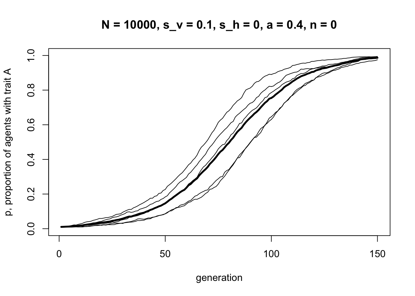
This should be roughly the same shape as the corresponding figure above with \(s_v = 0.1\) and \(a = 0.4\). Now let’s turn off vertical transmission and try just horizontal transmission:
data_model6c <- VerticalHorizontal(N = 10000,
                                   p_0 = 0.01,
                                   s_v = 0,
                                   s_h = 0.1,
                                   a = 0,
                                   n = 1,
                                   t_max = 150,
                                   r_max = 5)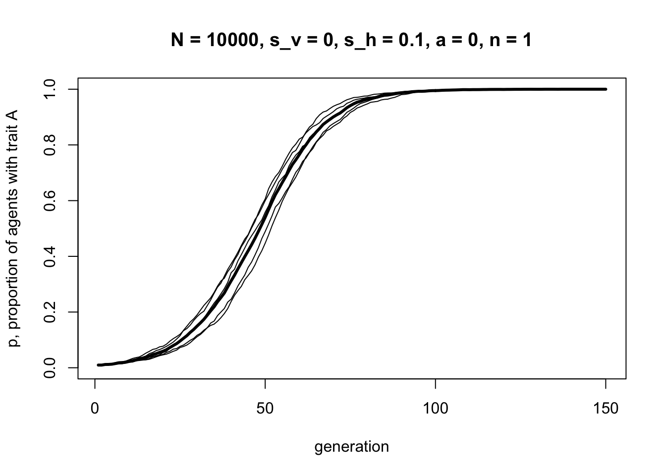
Horizontal transmission with \(s_h = 0.1\) and \(n = 1\) looks almost identical to the plot generated from BiasedTransmission in Model 3 with \(s = 0.1\). This makes sense because BiasedTransmission used the same rule, but with \(n\) fixed at one.
The curve above also looks almost identical to the first vertical transmission curve generated above in Model 6a using VerticalTransmission with \(s_v = 0.1\) and \(a = 0\). Under these assumptions, vertical cultural transmission from two randomly chosen parents is equivalent to horizontal cultural transmission from one randomly chosen demonstrator.
Now let’s increase \(n\), the number of demonstrators in horizontal transmission:
data_model6c <- VerticalHorizontal(N = 10000,
                                   p_0 = 0.01,
                                   s_v = 0,
                                   s_h = 0.1,
                                   a = 0,
                                   n = 5,
                                   t_max = 150,
                                   r_max = 5)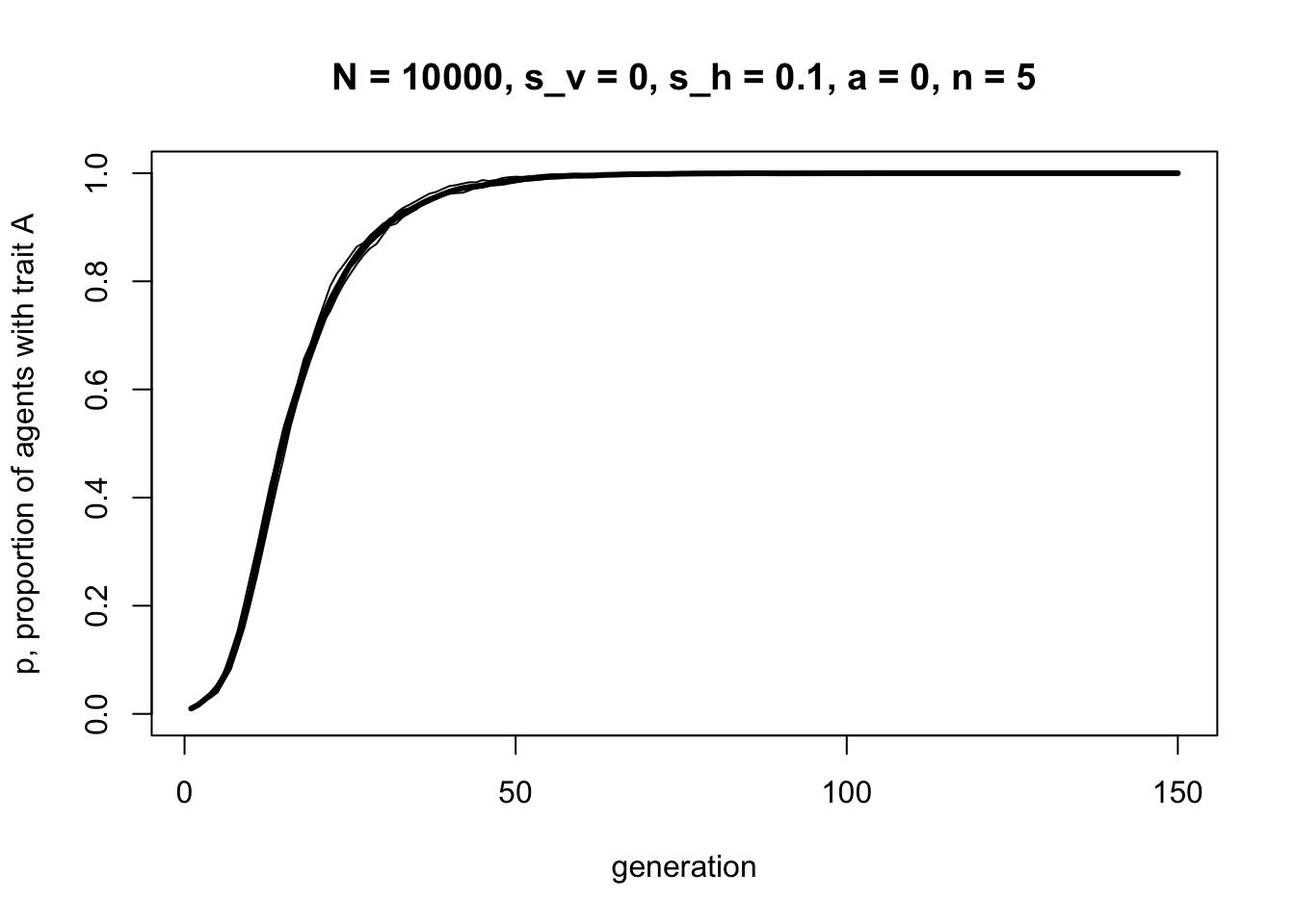
Increasing \(n\) greatly increases the strength of selection due to horizontal cultural transmission. If you only need one out of five demonstrators to have \(A\) for selection to operate, then selection for \(A\) will be more frequent than if you need one out of one demonstrator to have \(A\).
If we set \(-1 < s_v < 0\) then biased vertical transmission favours \(B\), rather than \(A\). Combining this with \(s_h > 0\) gives the case where vertical and horizontal transmission act in opposite directions. This might represent a ‘clash of the generations’ over traits such as smoking: parents exert pressure on children not to smoke, while peer pressure encourages smoking. The following illustrates such a case:
data_model6c <- VerticalHorizontal(N = 10000,
                                   p_0 = 0.01,
                                   s_v = -0.2,
                                   s_h = 0.1,
                                   a = 0.1,
                                   n = 5,
                                   t_max = 250,
                                   r_max = 5)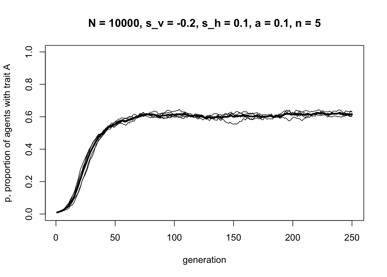
Whereas before there was always a single equilibrium at \(p = 1\), here there is a stable mix of \(A\) and \(B\) agents co-existing at equilibrium at a point where the vertical and horizontal transmission biases balance out. In the plot above, this equilibrium value is approximately \(p^* = 0.6\), but this varies with different combinations of \(s_v\), \(a\), \(s_h\) and \(n\).
We started this discussion by comparing vertical-only genetic inheritance with cultural inheritance, which can be horizontal as well as (or instead of) vertical. Let’s create a plot to compare three cases: vertical-only, horizontal-only and vertical-plus-horizontal. In each, vertical and horizontal transmission are now acting in the same direction, to favour trait \(A\). We are interested in how quickly this favoured trait \(A\) spreads and goes to fixation.
The following code runs these three scenarios with make_plot = FALSE to avoid automatically plotting the results. Instead we store the output from each case, and plot all three on the same graph using different colours and a legend.
data_model6c_v <- VerticalHorizontal(N = 10000,
                                     p_0 = 0.01,
                                     s_v = 0.1,
                                     s_h = 0,
                                     a = 0.1,
                                     n = 0,
                                     t_max = 150,
                                     r_max = 5,
                                     make_plot = FALSE)

data_model6c_h <- VerticalHorizontal(N = 10000,
                                     p_0 = 0.01,
                                     s_v = 0,
                                     s_h = 0.1,
                                     a = 0,
                                     n = 5,
                                     t_max = 150,
                                     r_max = 5,
                                     make_plot = FALSE)

data_model6c_vh <- VerticalHorizontal(N = 10000,
                                      p_0 = 0.01,
                                      s_v = 0.1,
                                      s_h = 0.1,
                                      a = 0.1,
                                      n = 5,
                                      t_max = 150,
                                      r_max = 5,
                                      make_plot = FALSE)

# plot vertical-only in blue
plot(rowMeans(data_model6c_v),
        type = 'l',
        ylab = "p, proportion of agents with trait A",
        xlab = "generation",
        ylim = c(0,1),
        lwd = 3,
        col = "royalblue")

for (r in 1:ncol(data_model6c_v)) {
  lines(data_model6c_v[,r], type = 'l', col = "royalblue")
}

# plot horizontal-only in orange
lines(rowMeans(data_model6c_h), type = 'l', lwd = 3, col = "orange")

for (r in 1:ncol(data_model6c_h)) {
  lines(data_model6c_h[,r], type = 'l', col = "orange")
}

# plot vertical-horizontal in grey
lines(rowMeans(data_model6c_vh), type = 'l', lwd = 3, col = "grey")

for (r in 1:ncol(data_model6c_vh)) {
  lines(data_model6c_vh[,r], type = 'l', col = "grey")
}

legend("bottomright",
       legend = c("Vertical transmission only",
                  "Horizontal transmission only",
                  "Vertical plus horizontal transmission"),
       lty = 1,
       lwd = 3,
       col = c("royalblue", "orange", "grey"),
       bty = "n")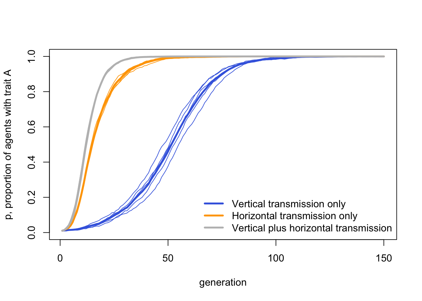
As we might expect, vertical plus horizontal transmission is fastest, with both forms of biased transmission combining together to favour \(A\). This is closely followed by horizontal transmission alone, which has the advantage of a large pool of demonstrators. The genetic-inheritance-like vertical transmission alone is slowest.
Summary
Our previous models all assumed oblique cultural transmission, where new agents learn from members of the previous generation. Here we modelled vertical cultural transmission, where agents learn from two parents (akin to genetic evolution), and horizontal cultural transmission, where agents learn from members of the same generation.
In Model 6a vertical cultural transmission was modelled in a simple way by picking two random members of the previous generation to be the parents for each new agent, then unbiased or biased transmission of traits occurs from those parents. This effectively recapitulated our previous unbiased and directly biased oblique transmission models but with slightly different assumptions. This consistency gives us confidence in the findings. It is always good to implement the same concept in different ways, to check that its effects are consistent or whether they depend on particular assumptions.
In Model 6b we extended vertical transmission by adding assortative mating, where the two parents are more culturally similar than expected under random mating. Assortative cultural mating acts in Model 6b to reduce the strength of cultural selection. This is because we assume that culturally identical parents always produce culturally identical offspring, and the selection bias only acts when parents have different traits. We can change these assumptions to explore other scenarios, and get different results (see Cavalli-Sforza & Feldman 1981). In general, assortative mating can potentially have positive effects, such as improving communication or cooperation between the parents thus making transmission more likely, or negative effects, such as generating cultural segregation or inequality in the population.
Finally, in Model 6c we implemented horizontal transmission, which we assume occurs after vertical transmission, is also directly biased, and occurs from \(n\) demonstrators in the same generation as the learner. Model 6c showed that the strength of directly biased horizontal transmission increases not only with the selection strength parameter \(s_h\), but also with \(n\). This reflects an often-cited advantage of horizontal over vertical transmission: one can potentially learn from many more sources than just your two parents.
When vertical and horizontal transmission act in different directions, i.e. to favour different traits, then we see a stable mixed equilibrium where \(A\) and \(B\) co-exist in the population. This might reflect a case where parents favour one cultural trait (e.g. not smoking), and peer-pressure favours a different trait (e.g. smoking). Whereas previously biased vertical and horizontal transmission both eliminate variation from the population, in this case cultural variation is maintained.
Model 6c showed that horizontal transmission can be faster at spreading favoured traits than vertical transmission, especially when there are many demonstrators from whom agents learn. Vertical plus horizontal transmission is faster still, assuming both act in the same direction. Empirically, vertical plus horizontal (or vertical plus oblique) transmission is thought to be typical of real life human cultural inheritance, with children initially learning from their parents then updating from peers and elders later in life (Aunger 2000; Henrich & Broesch 2011).
The empirical record also shows that, over long timescales, cultural evolution is faster than genetic evolution (Perreault 2012). It is likely that horizontal cultural transmission is responsible for this speed, and has allowed human populations to adapt culturally to novel environments faster than they would have been able to via vertical-only genetic evolution alone. When a novel trait emerges in a population via mutation or migration, whether it is the bow-and-arrow or the smart phone, horizontal transmission allows it to spread far faster than if transmission were purely vertical. On the other hand, horizontal transmission might also allow harmful traits to rapidly spread before their negative effects become known, or before natural selection has had a chance to act on them.
The models here can be extended to look at uniparental vertical transmission, where either the mother or father is more culturally influential, rather than the biparental transmission we implemented above. Some traits are known to be transmitted uniparentally, or more strongly by one parent than the other. For example, one survey of Stanford students in the early 1980s found that religious denomination was more strongly maternally transmitted, and political orientation more strongly paternally transmitted (Cavalli-Sforza et al. 1982). Uniparental transmission will exhibit different long-term dynamics than biparental transmission (see Cavalli-Sforza & Feldman 1981).
Note that there is a subtle difference between vertical and horizontal transmission in this model. For vertical transmission, we assume (quite reasonably) that children come into the world lacking any cultural traits. Consequently, the vertical transmission table above gives the probabilities of adopting either \(A\) or \(B\) given the parents’ values and the selection strength parameter \(s_v\). For horizontal transmission, on the other hand, children already have a cultural trait, the one they obtained as a result of vertical transmission. We assume that if they already have \(A\), there is no possibility of switching to \(B\). If they already have \(B\), then there is a chance of switching to \(A\), depending on \(s_h\) and whether any of the \(n\) demonstrators have \(A\). We can imagine here that individuals who have direct experience of \(A\) can be sure that it is better than \(B\), so never switch. Individuals with \(B\) need one exposure to \(A\) in order to learn it, and do so with probability \(s_h\). You might think that this unfairly weights the influence of horizontal transmission greater than that of vertical transmission. And that’s fine! You are welcome to modify the model to better match how you think the transmission pathways should work, or better match empirical data. That’s the beauty of models: because they are formally specified, it’s easy to see where you might disagree with assumptions (which are often hidden or implicit in verbal models) and change them.
In terms of programming techniques, there is not much new here. We have recycled code from several previous models, especially the directly biased transmission from Model 3 and the ‘mating table’ approach of Model 5. Don’t be afraid to re-use code, if it’s been tried and tested elsewhere (with appropriate attribution, if it’s not your own code). The one minor innovation was wrapping the plotting in a for statement and using a parameter make_plot to turn the automatic plotting on or off. This is useful if you want to combine plots from multiple runs, as we did in the final graph comparing the different pathways of inheritance.
Exercises
Try different values of \(s_v\) in VerticalTransmission to confirm that increasing \(s_v\) increases the speed with which \(A\) goes to fixation, and confirm that these dynamics are identical to how \(s\) acts in BiasedTransmission from Model 3.
Try running VerticalTransmission with \(s_v = -0.1\) and \(p_0 = 0.9\). What happens? What does a negative value of \(s_v\) mean?
Modify VerticalTransmission to allow the mother and the father to have different levels of influence. Replace the single \(s_v\) parameter with two selection parameters, one for the mother and one for the father. Explore the dynamics of uniparental biased transmission, compared to the biparental biased transmission implemented in the original model.
Try different values of \(a\) in VerticalAssortative to confirm that as \(a\) increases, selection slows. Write a function to record the number of timesteps it takes for a run to go to fixation (\(p=1\)) for different values of \(a\), and constant \(s_v\). Plot \(a\) against this measure.
Try different values of \(s_h\) and \(n\) in VerticalHorizontal to confirm that as both parameters increase, the speed with which \(A\) goes to fixation increases. Again, create plots to show how fixation time varies with \(s_h\) and with \(n\), with all other variables constant.
Try different negative values of \(s_v\), along with different values of \(a\), \(s_h\) and \(n\), to confirm that there are different mixed equilibria depending on the balance of vertical and horizontal transmission bias.
Rewrite VerticalHorizontal, replacing the horizontal cultural transmission rule with conformity, using code from Model 5. Does this change the conclusions regarding the speed of vertical vs horizontal transmission?
Analytic Appendix
Following Cavalli-Sforza & Feldman (1981, Table 2.2.1), we can write out the full mating table for two parents as follows. For simplicity, we assume that their \(b_3 = 1\), \(b_0 = 0\), and \(b_1 = b_2 = 1/2 + s/2\). In other words, there is no mutation and so two parents with the same trait always give rise to children with that trait, and when parental traits conflict then \(s_v\) represents the strength of selection for \(A\) under vertical transmission, irrespective of which parent the trait comes from.
| Mother’s trait | Father’s trait | Probability of child adopting \(A\) | Probability of pair forming under random mating | Probability of pair forming under assortative mating |
|---|---|---|---|---|
| \(A\) | \(A\) | 1 | \(p^2\) | \(p^2 + ap(1-p)\) |
| \(A\) | \(B\) | \(1/2 + s_v/2\) | \(p(1-p)\) | \(p(1-p)(1-a)\) |
| \(B\) | \(A\) | \(1/2 + s_v/2\) | \(p(1-p)\) | \(p(1-p)(1-a)\) |
| \(B\) | \(B\) | 0 | \((1-p)^2\) | \((1-p)^2 + ap(1-p)\) |
Considering random mating first, the frequency of \(p\) in the next generation, \(p'\), is given by multiplying the probability of a child adopting \(A\) (column 3) by the probability of a pair forming under random mating (column 4) for each parental trait combination, then summing these products. This gives
\[ p' = p^2 + (1+s_v)p(1-p)\]
which simplifies to
\[ p' = p + p(1-p)s_v \hspace{30 mm}(6.1)\]
This is identical to Equation 3.1 from Model 3 where there was a single randomly-selected demonstrator (i.e. one ‘parent’), rather than two. As in Equation 3.1, the change in \(p\) from one generation to the next is proportional to the strength of selection, \(s_v\), and the variance in \(p\), \(p(1 - p)\). In the Analytic Appendix to Model 3 we plotted this recursion to show that it takes the form of an s-shaped curve.
Following Cavalli-Sforza & Feldman (1981, Table 2.5.1) we can alternatively use the probability of a pair forming under assortative mating (column 5). (Note that I’ve used \(a\) rather than Cavalli-Sforza & Feldman’s \(m\) to avoid confusion with the migration parameter \(m\) used elsewhere.) As in the simulation model, a proportion \(a\) of matings are assortative, i.e. between two agents with the same cultural trait (either \(A\) and \(A\) or \(B\) and \(B\)), and \(1 - a\) matings are random as before. For example, for the first \(A\) x \(A\) row, there are \((1 - a)\) matings that are random and so have probability \(p^2\) as previously, and \(a\) matings that are assortative and will have probability \(p\) (because of the \(a\) matings that are assortative, the \(A\) x \(A\) pairings will occur with probability \(p\) and the \(B\) x \(B\) pairings will occur with probability \(1 - p\)). This gives:
\[ prob(A \text{ x } A) = (1-a)p^2 + ap = p^2 - ap^2 + ap = p^2 + ap(1-p) \hspace{30 mm}(6.2) \]
and so on for the other rows.
As for random mating, we then multiply and sum the third and fifth columns to get \(p'\) under assortative mating:
\[ p' = p^2 + ap(1-p) + (1+s_v)p(1-p)(1-a) \]
which simplifies to:
\[ p' = p + p(1-p)s_v(1-a) \hspace{30 mm}(6.3)\]
This is the same as Equation 6.1 but with the difference between \(p\) in successive generations also proportional to \((1 - a)\). That is, the larger is \(a\), the less change there is (at the extreme, \(a = 1\), then \(\Delta p = 0\)). Assortative mating acts against selection.
Finally we can introduce a recursion for horizontal transmission. As in the simulation model, we assume that individuals observe \(n\) individuals and adopt \(A\) with probability \(s_h\) if at least one of those \(n\) individuals possesses trait \(A\).
If \(p''\) denotes the frequency of \(A\) after horizontal transmission, and \(p'\) the frequency before horizontal transmission but after vertical transmission as per Equation 6.1 or 6.3, then:
\[ p'' = p' + (1-p')s_h(1 - (1-p')^n) \hspace{30 mm}(6.4)\]
Here, there are \(p'\) individuals who already have \(A\) and so can’t change, and \((1 - p')\) individuals who have \(B\) and change to \(A\) with probability equal to the strength of selection in horizontal transmission, \(s_h\), multiplied by the probability that at least one of the \(n\) demonstrators has an \(A\). This latter probability will be one minus the probability of none of the \(n\) individuals possessing \(A\), i.e. \(1 - (1 - p)^n\).
The potency of horizontal transmission lies in this last term. When \(n = 1\), then \(1 - (1 - p)^n\) reduces to \(p\), and we retrieve the same directly biased transmission form as Equations 3.1 and 6.1. As \(n\) increases, then \(1 - (1 - p)^n\) tends to 1. Because \(p\) must be less than or equal to 1, when \(n > 1\) then horizontal transmission must be stronger than vertical transmission, for identical selection strength parameters, until an equilibrium is reached at \(p = 1\) at which there is no change.
We can simulate the two recursions specified in Equations 6.3 and 6.4:
VerticalHorizontalRecursion <- function(s_v, a, s_h, n, t_max, p_0) {

  p <- rep(0,t_max)
  p[1] <- p_0

  for (i in 2:t_max) {

    p[i] <- p[i-1] + p[i-1]*(1-p[i-1])*s_v*(1-a)  # Eq 6.3

    p[i] <- p[i] + (1-p[i])*s_h*(1-(1-p[i])^n)  # Eq 6.4

  }

  plot(x = 1:t_max, y = p,
       type = "l",
       ylim = c(0,1),
       ylab = "p, frequency of A trait",
       xlab = "generation",
       main = paste("s_v = ", s_v, ", a = ", a, ", s_h = ", s_h, ", n = ", n, sep = ""))

  p # output p
}
The following code plots the recursion line in black and the simulation data with a grey dashed line, for the same parameter values specifying vertical transmission only. We increase \(r_{max}\) to 20 to make the simulation mean as accurate as possible. They should match pretty well, confirming that both our simulation code and our maths is correct.
recursion_data <- VerticalHorizontalRecursion(p_0 = 0.01,
                                              s_v = 0.1,
                                              s_h = 0,
                                              a = 0.4,
                                              n = 0,
                                              t_max = 150)

simulation_data <- VerticalHorizontal(N = 10000,
                                      p_0 = 0.01,
                                      s_v = 0.1,
                                      s_h = 0,
                                      a = 0.4,
                                      n = 0,
                                      t_max = 150,
                                      r_max = 20,
                                      make_plot = FALSE)

lines(rowMeans(simulation_data), col = "grey", lwd = 3, lty = 2)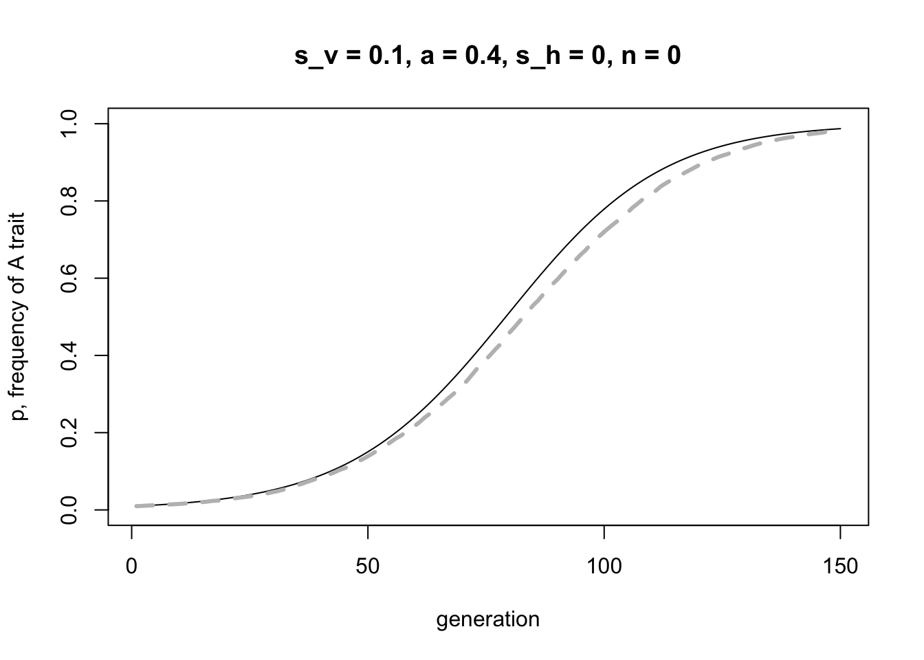
Here is the same for the case where vertical and horizontal transmission act in opposite directions:
recursion_data <- VerticalHorizontalRecursion(p_0 = 0.01,
                                              s_v = -0.2,
                                              s_h = 0.1,
                                              a = 0.1,
                                              n = 5,
                                              t_max = 150)

simulation_data <- VerticalHorizontal(N = 10000,
                                      p_0 = 0.01,
                                      s_v = -0.2,
                                      s_h = 0.1,
                                      a = 0.1,
                                      n = 5,
                                      t_max = 150,
                                      r_max = 20,
                                      make_plot = FALSE)

lines(rowMeans(simulation_data), col = "grey", lwd = 3, lty = 2)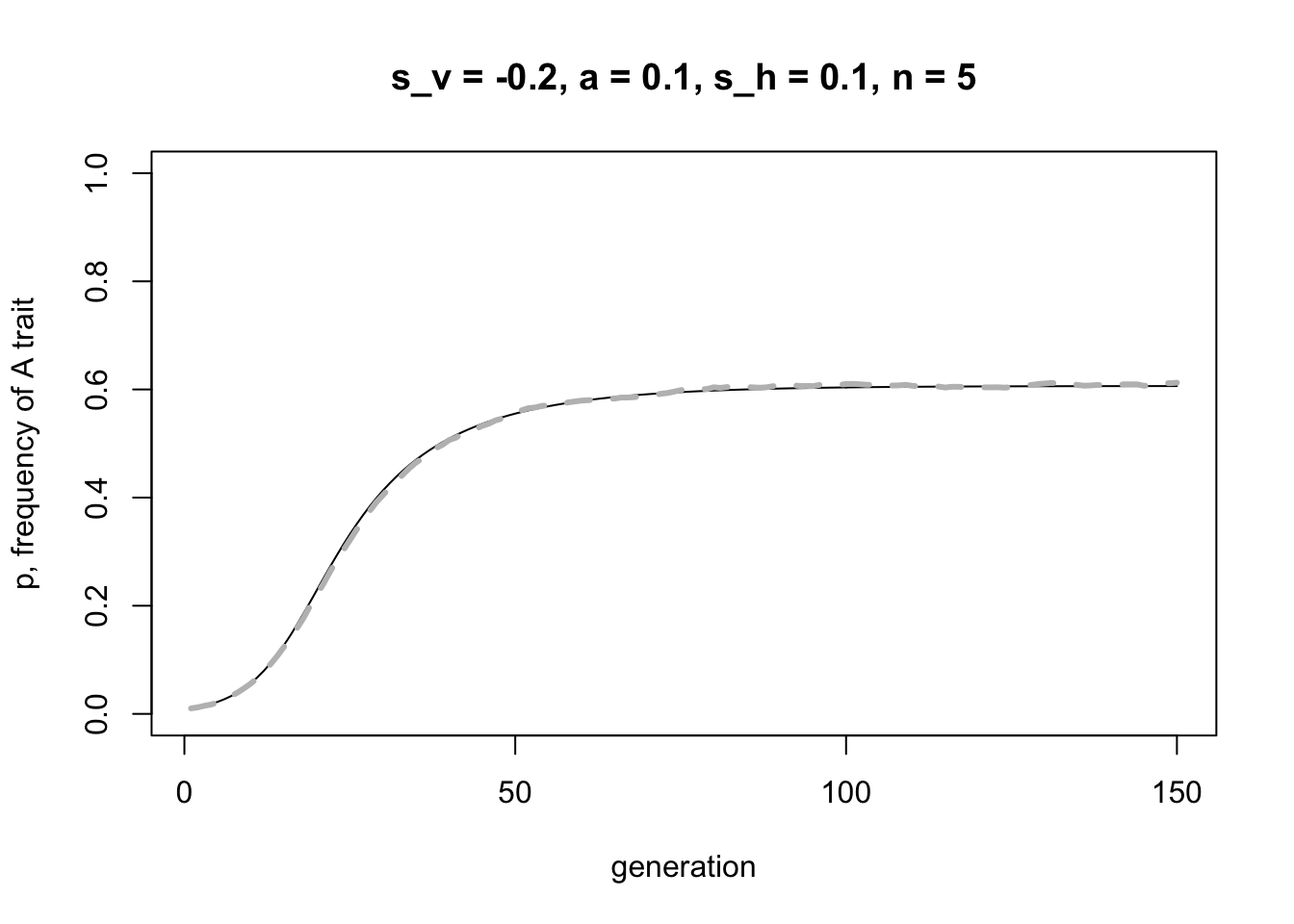
Again, a good match.
The equilibrium value \(p^*\) can be found when \(p = p''\). To make things easier, we can assume that \((1 - p')^n\) in Equation 6.4 is approximately zero when \(n\) is large, and so \((1 - (1 - p)^n)\) is approximately 1. Removing this term, substituting Equation 6.3 into 6.4, and setting \(p = p''\) gives:
\[ p = p + p(1-p)s_v(1-a) + s_h(1- (p + p(1-p)s_v(1-a)) ) \]
This can be rearranged to give:
\[ (1-p) (p (s_v(1-a) - s_h s_v(1-a)) + s_h) = 0 \hspace{30 mm}(6.5)\]
Hence there is one equilibrium when the first term \(1 - p = 0\), such that \(p^* = 1\). There is another where
\[ p (s_v(1-a) - s_h s_v(1-a)) + s_h = 0 \]
which rearranges to give
\[ p^* = -\frac{s_h} {(1-a) (s_v - s_h s_v)} \hspace{30 mm}(6.6)\]
With the values used in the previous graph, we can use Equation 6.6 to find the value of the internal equilibrium that we observed:
## [1] 0.617284This should approximately match the final values of both the simulation and recursion data:
## [1] 0.612535## [1] 0.606279It’s not an exact match due to the removal of the term with \(n\). The match should get better as \(n\) increases.
Given that \(p^*\) must be less than one, an internal equilibrium can only exist when the right hand side of Equation 6.6 is less than one. After rearranging, this gives the inequality:
\[ s_v (1-a) < -\frac {s_h} {(1-s_h)} \hspace{30 mm}(6.7)\]
Because \(s_h\) must be positive by assumption, the right hand side of Equation 6.7 must be negative. Consequently the inequality in Equation 6.7 can only be true when \(s_v\) is negative, and moreover negative enough (after being reduced in strength by assortative cultural mating) to outweigh \(s_h\) acting in the opposite direction.
References
Aunger, R. (2000). The life history of culture learning in a face‐to‐face society. Ethos, 28(3), 445-481.
Cavalli-Sforza, L. L., & Feldman, M. W. (1981). Cultural transmission and evolution: a quantitative approach. Princeton University Press.
Cavalli-Sforza, L. L., Feldman, M. W., Chen, K. H., & Dornbusch, S. M. (1982). Theory and observation in cultural transmission. Science, 218(4567), 19-27.
Henrich, J., & Broesch, J. (2011). On the nature of cultural transmission networks: evidence from Fijian villages for adaptive learning biases. Philosophical Transactions of the Royal Society B, 366(1567), 1139-1148.
Perreault, C. (2012). The pace of cultural evolution. PLoS One, 7(9), e45150.