Model 2: Unbiased and biased mutation
Introduction
Evolution doesn’t work without a source of variation that introduces new variation upon which selection, drift and other processes can act. In genetic evolution, mutation is almost always blind with respect to function. Beneficial genetic mutations are no more likely to arise when they are needed than when they are not needed - in fact most genetic mutations are neutral or detrimental to an organism. Cultural evolution is more interesting, in that novel variation may sometimes be directed to solve specific problems, or systematically biased due to features of our cognition. In the models below we’ll simulate both unbiased and biased mutation.
Model 2a: Unbiased mutation
First we will simulate unbiased mutation in the same basic model as used in Model 1 (Unbiased transmission). We’ll remove unbiased transmission to see the effect of unbiased mutation alone.
As in Model 1, we assume \(N\) individuals each of whom possesses one of two cultural traits, denoted \(A\) and \(B\). In each generation from \(t = 1\) to \(t = t_{max}\), the \(N\) agents are replaced with \(N\) new agents. Instead of random copying, each agent now gives rise to a new agent with exactly the same cultural trait as them. (Another way of looking at this is in terms of timesteps, such as years: the same \(N\) agents live for \(t_{max}\) years, and keep their cultural trait from one year to the next.)
Each generation, there is a probability \(\mu\) that each agent mutates from their current trait to the other trait. This probability applies to each agent independently; whether an agent mutates has no bearing on whether or how many other agents have mutated. On average, that means that \(\mu N\) agents mutate each generation. Like in Model 1, we are interested in tracking the proportion \(p\) of agents with trait \(A\) over time.
We’ll wrap this in a function called UnbiasedMutation, using much of the same code as UnbiasedTransmission. Now though we have an extra parameter, \(\mu\), to specify.
UnbiasedMutation <- function (N, mu, p_0, t_max, r_max) {

  # create a matrix with t_max rows and r_max columns, fill with NAs, convert to dataframe
  output <- as.data.frame(matrix(NA, t_max, r_max))

  # purely cosmetic: rename the columns with run1, run2 etc.
  names(output) <- paste("run", 1:r_max, sep="")

  for (r in 1:r_max) {

    # create first generation
    agent <- data.frame(trait = sample(c("A","B"), N, replace = TRUE,
                        prob = c(p_0,1-p_0)))

    # add first generation's p to first row of column r
    output[1,r] <- sum(agent$trait == "A") / N

    for (t in 2:t_max) {

      # copy agent to previous_agent dataframe
      previous_agent <- agent

      # get N random numbers each between 0 and 1
      mutate <- runif(N)

      # if agent was A, with probability mu, flip to B
      agent$trait[previous_agent$trait == "A" & mutate < mu] <- "B"

      # if agent was B, with probability mu, flip to A
      agent$trait[previous_agent$trait == "B" & mutate < mu] <- "A"

      # get p and put it into output slot for this generation t and run r
      output[t,r] <- sum(agent$trait == "A") / N

    }

  }

  # first plot a thick line for the mean p
  plot(rowMeans(output),
       type = 'l',
       ylab = "p, proportion of agents with trait A",
       xlab = "generation",
       ylim = c(0,1),
       lwd = 3,
       main = paste("N = ", N, ", mu = ", mu, sep = ""))

  for (r in 1:r_max) {

    # add lines for each run, up to r_max
    lines(output[,r], type = 'l')

  }

  output  # export data from function
}
The only changes from Model 1 are the addition of \(\mu\) in the function definition and the plot title, and three new lines of code within the \(t\) for loop which replace the random copying command with unbiased mutation. Let’s examine these three lines to see how they work.
The most obvious way of implementing unbiased mutation - which is NOT done above - would have been to set up another for loop. We would cycle through each agent one by one, each time calculating whether it should mutate or not based on \(/mu\). This would certainly work, but R is notoriously slow at loops. It’s always preferable in R, where possible, to use ‘vectorised’ code. That’s what is done above in our three added lines.
First we pre-specify the probability of mutating for each agent. This is done with the runif (random draws from a uniform distribution) command which generates \(N\) random numbers each between 0 and 1, and puts them into a variable called mutate. If the ith value in mutate is less than or equal to \(\mu\), then the ith agent in our agent dataframe will mutate. This is done on the subsequent two lines, first for agents that were previously \(A\), and then for agents that were previously \(B\).
We can think about this by imagining what happens at extreme values of \(\mu\). If \(\mu = 1\), then that agent’s mutate value will always be less than \(\mu\), because the maximum value of mutate is 1 (we can ignore the case when mutate happens to be exactly 1.000, as it will very rarely happen). The inequality is therefore always true, and the agent always mutates. That’s what we want to happen, if \(\mu = 1\). The following code illustrates this:
N <- 100
mu <- 1  # maximum mutation rate of 1

# get N random numbers each between 0 and 1
mutate <- runif(N)

# always mutate
mutate < mu
## [1] TRUE TRUE TRUE TRUE TRUE TRUE TRUE TRUE TRUE TRUE TRUE TRUE TRUE TRUE TRUE
## [16] TRUE TRUE TRUE TRUE TRUE TRUE TRUE TRUE TRUE TRUE TRUE TRUE TRUE TRUE TRUE
## [31] TRUE TRUE TRUE TRUE TRUE TRUE TRUE TRUE TRUE TRUE TRUE TRUE TRUE TRUE TRUE
## [46] TRUE TRUE TRUE TRUE TRUE TRUE TRUE TRUE TRUE TRUE TRUE TRUE TRUE TRUE TRUE
## [61] TRUE TRUE TRUE TRUE TRUE TRUE TRUE TRUE TRUE TRUE TRUE TRUE TRUE TRUE TRUE
## [76] TRUE TRUE TRUE TRUE TRUE TRUE TRUE TRUE TRUE TRUE TRUE TRUE TRUE TRUE TRUE
## [91] TRUE TRUE TRUE TRUE TRUE TRUE TRUE TRUE TRUE TRUEIf \(\mu = 0\), then that agent’s mutate value will never be less than \(\mu\), because the minimum value of mutate is 0. The inequality is therefore never true, and the agent never mutates. Again, that’s what we want, if \(\mu = 0\). In code:
N <- 100
mu <- 0  # minimum mutation rate of 0

# get N random numbers each between 0 and 1
mutate <- runif(N)

# never mutate
mutate < mu
## [1] FALSE FALSE FALSE FALSE FALSE FALSE FALSE FALSE FALSE FALSE FALSE FALSE
## [13] FALSE FALSE FALSE FALSE FALSE FALSE FALSE FALSE FALSE FALSE FALSE FALSE
## [25] FALSE FALSE FALSE FALSE FALSE FALSE FALSE FALSE FALSE FALSE FALSE FALSE
## [37] FALSE FALSE FALSE FALSE FALSE FALSE FALSE FALSE FALSE FALSE FALSE FALSE
## [49] FALSE FALSE FALSE FALSE FALSE FALSE FALSE FALSE FALSE FALSE FALSE FALSE
## [61] FALSE FALSE FALSE FALSE FALSE FALSE FALSE FALSE FALSE FALSE FALSE FALSE
## [73] FALSE FALSE FALSE FALSE FALSE FALSE FALSE FALSE FALSE FALSE FALSE FALSE
## [85] FALSE FALSE FALSE FALSE FALSE FALSE FALSE FALSE FALSE FALSE FALSE FALSE
## [97] FALSE FALSE FALSE FALSEAt intermediate values, say \(\mu = 0.1\), then the inequality is true for 10% of the mutate values, or in other words for 10% of the agents. Again, in code:
N <- 100
mu <- 0.1  # mutation rate of 10%

# get N random numbers each between 0 and 1
mutate <- runif(N)

# 10% of agents mutate
mutate < mu
## [1] FALSE FALSE FALSE FALSE TRUE FALSE FALSE FALSE TRUE TRUE FALSE FALSE
## [13] FALSE FALSE FALSE FALSE FALSE FALSE FALSE FALSE FALSE FALSE FALSE FALSE
## [25] FALSE FALSE FALSE FALSE FALSE TRUE FALSE FALSE FALSE FALSE FALSE FALSE
## [37] FALSE FALSE FALSE FALSE FALSE FALSE FALSE FALSE FALSE TRUE FALSE FALSE
## [49] FALSE FALSE FALSE FALSE FALSE FALSE FALSE FALSE FALSE TRUE TRUE FALSE
## [61] TRUE FALSE FALSE FALSE FALSE FALSE TRUE FALSE FALSE FALSE FALSE FALSE
## [73] FALSE FALSE FALSE FALSE FALSE FALSE FALSE FALSE FALSE FALSE FALSE FALSE
## [85] FALSE FALSE FALSE FALSE FALSE FALSE FALSE FALSE FALSE FALSE FALSE FALSE
## [97] FALSE FALSE FALSE FALSE## [1] 0.09The value gives the proportion of mutating agents, and should be approximately (not necessarily exactly) 0.1.
Let’s run this unbiased mutation model.
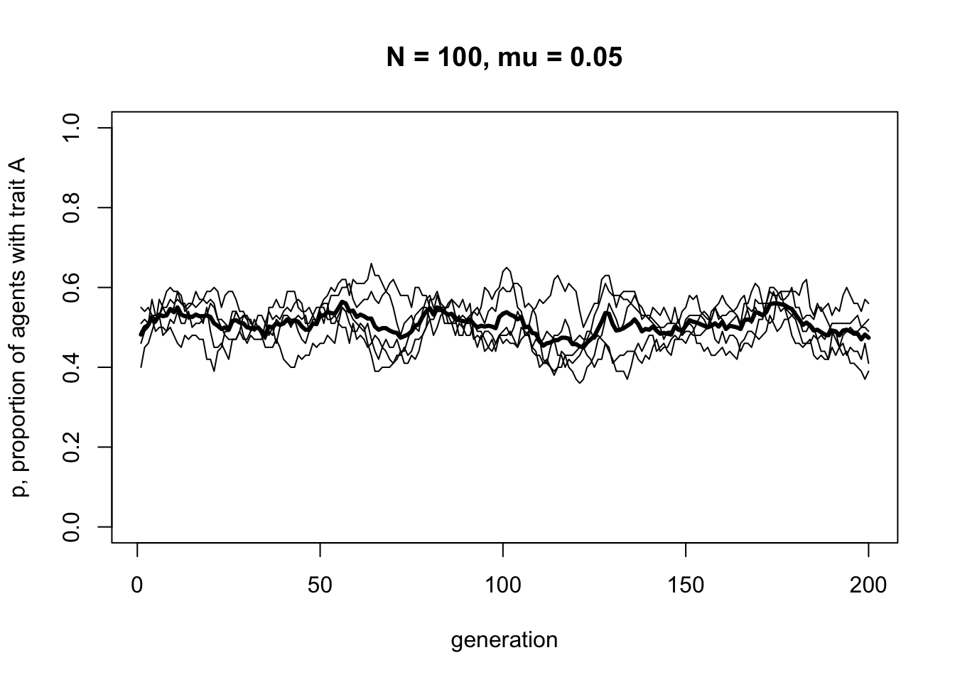
As one might expect, unbiased mutation produces random fluctuations over time, and does not alter the overall frequency of \(A\) which stays around \(p = 0.5\). Because mutations from \(A\) to \(B\) are as equally likely as \(B\) to \(A\), there is no overall directional trend.
But what if we were to start at different initial frequencies of \(A\) and \(B\)? Say, \(p = 0.2\) or \(p = 0.9\)? Would unbiased mutation keep \(p\) at these initial values, like we saw unbiased transmission does in Model 1?
To find out, let’s change \(p_0\), which, as you may recall from Model 1, specifies the initial probability of drawing an \(A\) rather than a \(B\) in the first generation.
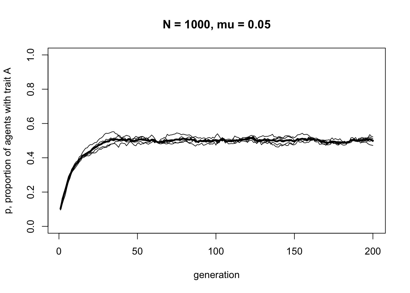
You should see \(p\) go from 0.1 up to 0.5. In fact, whatever the initial starting frequencies of \(A\) and \(B\), unbiased mutation always leads to \(p = 0.5\). Unlike the unbiased transmission simulated in Model 1, with unbiased mutation it is impossible for one trait to be lost and the other go to fixation. Unbiased mutation introduces and maintains cultural variation in the population.
Model 2b: Biased mutation
A more interesting case is biased mutation. Let’s assume now that there is a probability \(\mu_b\) that an agent with trait \(B\) mutates into \(A\), but there is no possibility of trait \(A\) mutating into trait \(B\). Perhaps trait \(A\) is a particularly catchy or memorable version of a story, or an intuitive explanation of a phenomenon, and \(B\) is difficult to remember or unintuitive.
The function BiasedMutation captures this unidirectional mutation.
BiasedMutation <- function (N, mu_b, p_0, t_max, r_max) {

  # create a matrix with t_max rows and r_max columns, fill with NAs, convert to dataframe
  output <- as.data.frame(matrix(NA, t_max, r_max))

  # purely cosmetic: rename the columns with run1, run2 etc.
  names(output) <- paste("run", 1:r_max, sep="")

  for (r in 1:r_max) {

    # create first generation
    agent <- data.frame(trait = sample(c("A","B"), N, replace = TRUE,
                        prob = c(p_0,1-p_0)))

    # add first generation's p to first row of column r
    output[1,r] <- sum(agent$trait == "A") / N

    for (t in 2:t_max) {

      # copy agent to previous_agent dataframe
      previous_agent <- agent

      # get N random numbers each between 0 and 1
      mutate <- runif(N)

      # if agent was B, with prob mu_b, flip to A
      agent$trait[previous_agent$trait == "B" & mutate < mu_b] <- "A"

      # get p and put it into output slot for this generation t and run r
      output[t,r] <- sum(agent$trait == "A") / N

    }

  }

  # first plot a thick line for the mean p
  plot(rowMeans(output),
       type = 'l',
       ylab = "p, proportion of agents with trait A",
       xlab = "generation",
       ylim = c(0,1),
       lwd = 3,
       main = paste("N = ", N, ", mu = ", mu_b, sep = ""))

  for (r in 1:r_max) {

    # add lines for each run, up to r_max
    lines(output[,r], type = 'l')

  }

  output  # export data from function
}
There are just two changes in this code compared to UnbiasedMutation. First, we’ve replaced \(\mu\) with \(\mu_b\) to keep the two parameters distinct and avoid confusion. Second, the line in UnbiasedMutation which caused agents with \(A\) to mutate to \(B\) has been deleted.
Let’s see what effect this has by running BiasedMutation. We’ll start with the population entirely composed of agents with \(B\), i.e. \(p_0 = 0\), to see how quickly and in what manner \(A\) spreads via biased mutation.
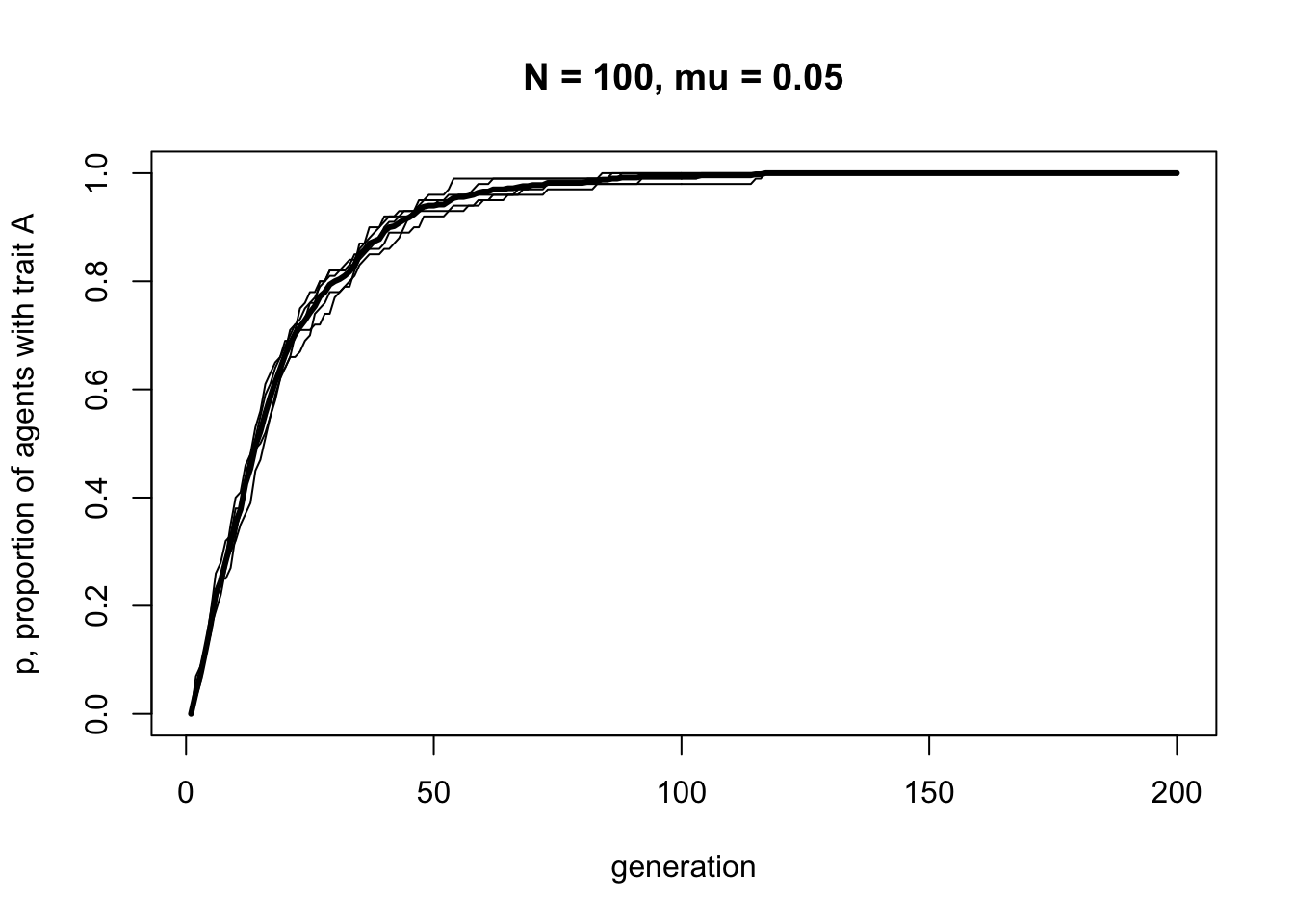
The plot should show a steep increase that slows and plateaus at \(p = 1\) by around generation \(t = 100\). There should be a bit of fluctuation in the different runs, but not much. Now let’s try a larger sample size.
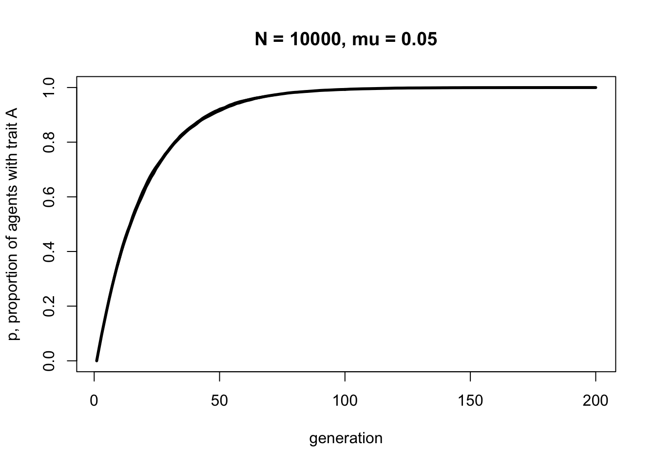
With \(N = 10000\) the line should be smooth with little fluctuation across the runs. But notice that it plateaus at about the same generation, around \(t = 100\). Population size has little effect on the rate at which a novel trait spreads via biased mutation. \(\mu_b\), on the other hand, does affect this speed. Let’s double the biased mutation rate to 0.1.
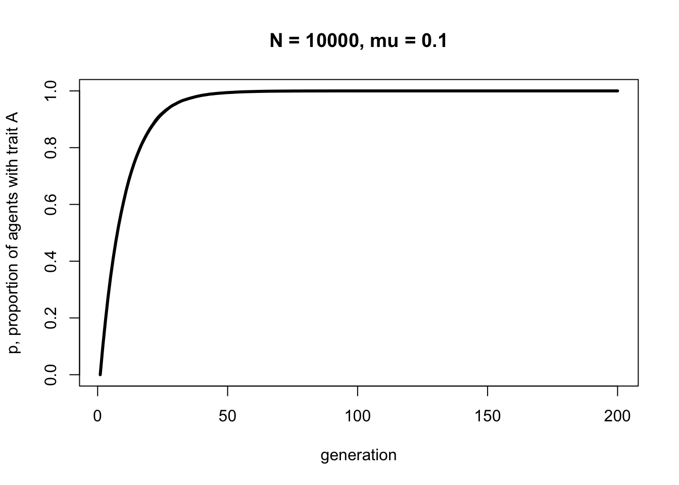
Now trait \(A\) reaches fixation around generation \(t = 50\). Play around with \(N\) and \(\mu_b\) to confirm that the latter determines the rate of diffusion of trait \(A\), and that it takes the same form each time - roughly an ‘r’ shape with an initial steep increase followed by a plateauing at \(p = 1\).
Summary
With this simple model we can draw the following insights. Unbiased mutation, which resembles genetic mutation in being non-directional, always leads to an equal mix of the two traits. It introduces and maintains cultural variation in the population. It is interesting to compare unbiased mutation to unbiased transmission from Model 1. While unbiased transmission did not change \(p\) over time, unbiased mutation always converges on \(p^* = 0.5\), irrespective of the starting frequency. (NB \(p^* = 0.5\) assuming there are two traits; more generally, \(p^* = 1/v\), where \(v\) is the number of traits.)
Biased mutation, which is far more common - perhaps even typical - in cultural evolution, shows different dynamics. Novel traits favoured by biased mutation spread in a characteristic fashion - an r-shaped diffusion curve - with a speed characterised by the mutation rate \(\mu_b\). Population size has little effect, whether \(N = 100\) or \(N = 10000\). This is because mutation is an individual-level process, and does not depend on the traits of any other agent(s) in the population. Whenever biased mutation is present (\(\mu_b > 0\)), the favoured trait goes to fixation, even if it is not initially present.
A form of unbiased cultural mutation can be observed when people try to copy artifact sizes or shapes, and the limits of our perceptual systems introduces random noise into the copied form. This has been studied in the context of the transmission of archaeological artifacts such as handaxes and arrowheads (Eerkens & Lipo 2005) and confirmed experimentally (Kempe et al. 2012).
Biased cultural mutation has been argued to result from universal features of human cognition, as different people or groups independently transform cultural traits towards certain ‘attractive’ forms. For example, studies have shown how portraits of subjects averting their gaze systematically mutated into portraits of subjects with direct eye gaze (Morin 2013), and how blood-letting as a medical practice independently emerged in different societies around the world (Miton et al. 2015).
In terms of programming techniques, the major novelty in Model 2 is the use of runif to generate a series of \(N\) random numbers from 0 to 1 and compare these to a fixed probability (in our case, \(\mu\) or \(\mu_b\)) to determine which agents should undergo whatever the fixed probability specifies (in our case, mutation). This could be done with a loop, but vectorising code in the way we did here is much faster in R than loops.
Exercises
Try different values of \(p_0\) in UnbiasedMutation to confirm that any starting value converges on approximately \(p=0.5\).
Try different values of \(p_0\) in BiasedMutation to confirm that any starting value converges on \(p=1\).
Try different values of \(N\) and \(\mu_b\) in BiasedMutation to confirm that \(\mu_b\) does, and \(N\) does not, affect the speed with which \(p\) reaches fixation.
Create an alternative UnbiasedMutation function which uses a for-loop to cycle through each agent and, for each one, mutate its cultural trait with probability \(\mu\). Use the function system.time() to compare the time that this looping function takes with the time the original vectorised UnbiasedMutation function takes, for the same parameter values. Is the vectorised version faster? If so, how many times faster?
Add a parameter \(\mu_a\) to BiasedMutation which determines the probability that an agent with \(A\) mutates to \(B\). Run the simulation to show that the equilibrium value of \(p\), and the speed at which this equilibrium is reached, depends on the difference between \(mu_a\) and \(mu_b\).
Add a third trait, \(C\), to the UnbiasedMutation function. The first generation should have traits set using sample with c(“A”, “B”, “C”) rather than c(“A”, “B”). You will need to define a new parameter, \(q_0\), which gives the probability of drawing a \(B\), equivalent to how \(p_0\) gives the probability of drawing an \(A\). The probability of drawing a \(C\) is then \(1 - p_0 - q_0\), given that all the probabilities have to add up to one. These probabilities can be entered into the prob argument of sample. Then modify the unbiased mutation lines such that, if an agent has trait \(A\), with probability \(\mu\) they have an equal chance of mutating into either \(B\) or \(C\); agents with trait \(B\) similarly have a probability \(\mu\) of mutating into either \(A\) or \(C\); and agents with \(C\) mutate with probability \(\mu\) into either \(A\) or \(B\). Record and plot \(p\), the frequency of \(A\), as before. Does \(p\) still converge on 0.5, as it does with only two traits?
Analytical Appendix
If \(p\) is the frequency of \(A\) in one generation, we are interested in calculating \(p'\), the frequency of \(A\) in the next generation under the assumption of unbiased mutation. The next generation retains the cultural traits of the previous generation, except that \(\mu\) of them switch to the other trait. There are therefore two sources of \(A\) in the next generation: members of the previous generation who had \(A\) and didn’t mutate, therefore staying \(A\), and members of the previous generation who had \(B\) and did mutate, therefore switching to \(A\). The frequency of \(A\) in the next generation is therefore:
\[p' = p(1 - \mu) + (1 - p) \mu \hspace{30 mm}(2.1)\]
The first term on the right-hand side of Equation 2.1 represents the first group, the \((1 - \mu)\) proportion of the \(p\) \(A\)-carriers who didn’t mutate. The second term represents the second group, the \(\mu\) proportion of the \(1 - p\) \(B\)-carriers who did mutate.
To calculate the equilibrium value of \(p\), \(p^*\), we want to know when \(p' = p\), or when the frequency of \(A\) in one generation is identical to the frequency of \(A\) in the next generation. This can be found by setting \(p' = p\) in Equation 2.1, which gives:
\[p = p(1-\mu) + (1-p)\mu \hspace{30 mm}(2.2)\]
Rearranging Equation 2.2 gives:
\[\mu(1 - 2p) = 0 \hspace{30 mm}(2.3)\]
The left-hand side of Equation 2.3 equals zero when either \(\mu = 0\), which given our assumption that \(\mu > 0\) cannot be the case, or when \(1 - 2p = 0\), which after rearranging gives the single equilibrium \(p^* = 0.5\). This matches our simulation results above. As we found in the simulations, this does not depend on \(\mu\) or the starting frequency of \(p\).
We can also plot the recursion in Equation 2.1 like so:
p_0 <- 0
t_max <- 200
mu <- 0.1

p <- rep(NA, t_max)
p[1] <- p_0

for (i in 2:t_max) {
  p[i] <- p[i-1]*(1 - mu) + (1-p[i-1])*mu
}

plot(p,
     type = 'l',
     ylab = "p, proportion of agents with trait A",
     xlab = "generation",
     ylim = c(0,1),
     lwd = 3)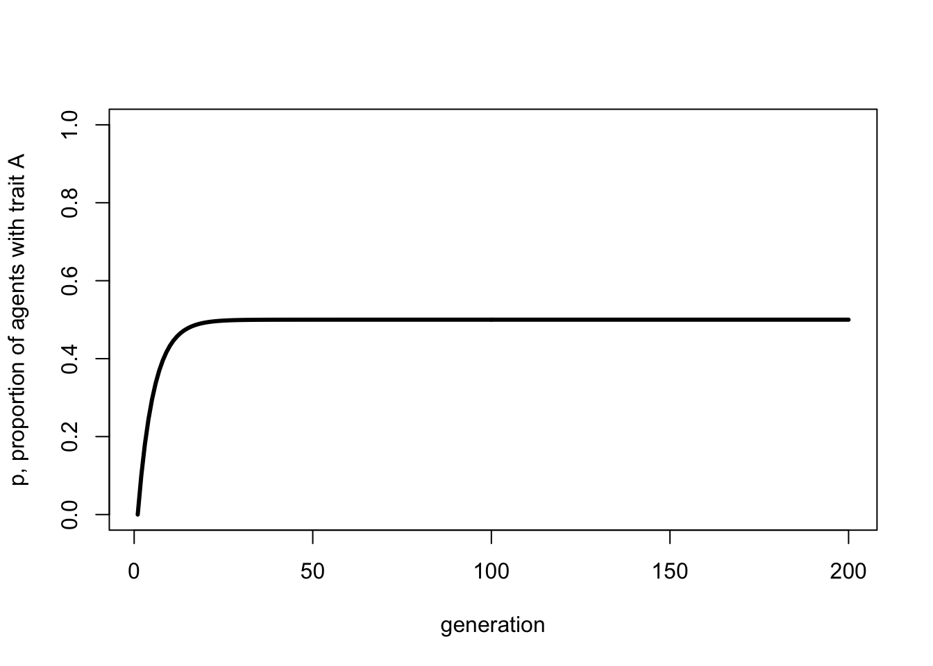
This should resemble the figure generated by the simulations above, and confirm that \(p^* = 0.5\).
For biased mutation, assume that only \(B\)s are switching to \(A\), and with probability \(\mu_b\) instead of \(\mu\). The first term on the right hand side becomes simply \(p\), because \(A\)s do not switch. The second term remains the same, but with \(\mu_b\). Thus,
\[p' = p + (1 - p) \mu_b \hspace{30 mm}(2.4)\]
The equilibrium value \(p^*\) can be found by again setting \(p' = p\) and solving for \(p\). Assuming \(\mu_b > 0\), this gives the single equilibrium \(p^* = 1\), which again matches the simulation results.
We can plot the above recursion like so:
p_0 <- 0
t_max <- 200
mu_b <- 0.1

p <- rep(NA, t_max)
p[1] <- p_0

for (i in 2:t_max) {
  p[i] <- p[i-1] + (1 - p[i-1])*mu_b
}

plot(p,
     type = 'l',
     ylab = "p, proportion of agents with trait A",
     xlab = "generation",
     ylim = c(0,1),
     lwd = 3)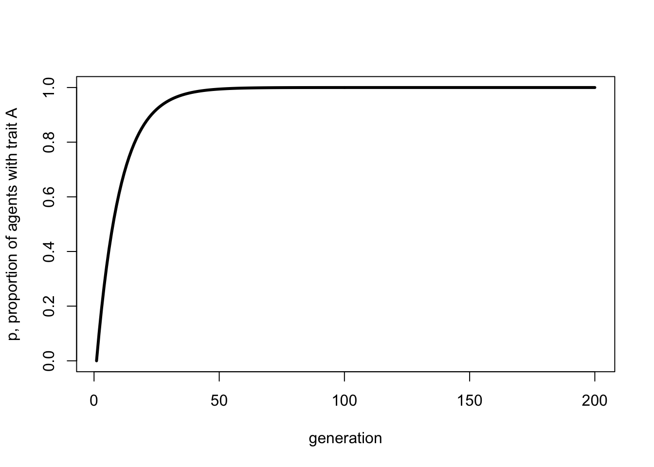
Hopefully, this looks identical to the final simulation plot with the same value of \(\mu_b\).
Furthermore, we can specify an equation for the change in \(p\) from one generation to the next, or \(\Delta p\). We do this by subtracting \(p\) from both sides of Equation 2.4, giving:
\[\Delta p = p' - p = (1 - p) \mu_b \hspace{30 mm}(2.5)\]
Seeing this helps explain two things. First, the \(1 - p\) part explains the r-shape of the curve. It says that the smaller is \(p\), the larger \(\Delta p\) will be. This explains why \(p\) increases in frequency very quickly at first, when \(p\) is near zero, and the increase slows when \(p\) gets larger. We have already determined that the increase stops altogether (i.e. \(\Delta p\) = 0) when \(p = p^* = 1\).
Second, it says that the rate of increase is proportional to \(\mu_b\). This explains our observation in the simulations that larger values of \(\mu_b\) cause \(p\) to reach its maximum value faster.
References
Eerkens, J. W., & Lipo, C. P. (2005). Cultural transmission, copying errors, and the generation of variation in material culture and the archaeological record. Journal of Anthropological Archaeology, 24(4), 316-334.
Kempe, M., Lycett, S., & Mesoudi, A. (2012). An experimental test of the accumulated copying error model of cultural mutation for Acheulean handaxe size. PLoS One, 7(11), e48333.
Miton, H., Claidière, N., & Mercier, H. (2015). Universal cognitive mechanisms explain the cultural success of bloodletting. Evolution and Human Behavior, 36(4), 303-312.
Morin, O. (2013). How portraits turned their eyes upon us: visual preferences and demographic change in cultural evolution. Evolution and Human Behavior, 34(3), 222-229.