Model 12: Historical dynamics
Introduction
As discussed in the context of Model 11 (Cultural Group Selection), cooperation is crucial to the functioning of large human societies. While Model 11 was all about how cooperation emerges within groups, in Model 12 we will zoom out to examine how cooperation, specifically the mechanism of cultural group selection, can determine broader historical dynamics at the level of the group and above.
In particular, we are interested in how large multi-group societies, or empires, rise and fall throughout human history. The rise and fall of empires is a standard historical pattern. At any point in history many empires exist. These empires compete with one another, some growing and becoming dominant for a time (think the Roman Empire), and all eventually collapsing (again, like the Roman Empire). Unlike in our previous models, there are no stable equilibria in human history. The ‘best’ empire or empires (whatever ‘best’ might mean) do not reach a stable size and stay there. Rather, there are continual oscillations, with new empires constantly emerging and growing, and existing empires constantly declining and disappearing. These dynamics are also often described as chaotic, in that it is virtually impossible to predict at any one time point exactly which empires will subsequently grow or collapse. Nevertheless, the overall dynamics of multiple co-existing, competing states going through cycles of emergence, dominance and collapse are worthy of explanation.
Turchin (2003) presented a cultural evolutionary theory of how empires rise and fall through human history. Turchin’s theory drew on the notion of cultural group selection (see Model 11), but combined this with historical detail concerning the various pressures acting on real empires from history. In Model 12 we will recapitulate the spatially explicit agent-based simulation of this theory from Chapter 4 of Turchin’s (2003) book.
One key element of Turchin’s (2003) cultural evolutionary theory of historical dynamics is the concept of asabiya. This term was coined by 14th century Islamic scholar Ibn Khaldun to describe the degree of within-group cooperation, or collective solidarity, possessed by a group. Members of groups high in asabiya generate public goods together, fight for one another, defend each other, monitor and punish free-riders, and generally engage in the kind of costly cooperative acts described in Model 11. Members of groups low in asabiya free-ride on each other, desert during conflicts, shirk costly punishment of free-riders, and engage in other non-cooperative acts. As in Model 11, groups higher in asabiya do better in intergroup conflict than groups lower in asabiya. This is cultural group selection.
A second key element of Turchin’s (2003) theory is the importance of frontier regions. These are regions where different empires or groups of different ethnicities meet. Turchin argues that asabiya is highest at these frontiers because of the presence and threat of competing groups. As modern day examples, religious beliefs tend to be stronger in regions like Northern Ireland or the Middle East where different competing religions exist in close proximity, compared to more religiously homogenous regions.
Turchin’s theory works as follows. In frontier regions, small groups high in asabiya engage in frequent intergroup conflict. Eventually one of these groups expands and takes over rival groups, becoming a multi-group empire. As this empire expands, its internal non-frontier region gets larger, causing the empire’s overall asabiya to drop. At the frontiers, new groups emerge that are high in asabiya. One of these grows big enough to invade the previous empire, which is weakened by its low asabiya. The new empire thus replaces the old empire. The new empire grows larger, its asabiya drops, and it in turn is invaded by a new empire that has emerged at its frontier. This cycle continues, generating the oscillatory dynamics characteristic of real human history.
Model 12
Model 12 simulates this process. The agents in Model 12 are groups. Individuals within groups are not explicitly modelled. Each group exists in one fixed position within an \(N_{side}\) x \(N_{side}\) square grid, like in Model 10 (Polarisation). Groups can either be independent entities existing outside of any empire, or they can belong to an empire. Each empire is denoted by a number, e.g. Empire 1, Empire 2 and so on. We use a matrix called \(E\) to store the empire id of each group: 0 indicates no empire, a positive integer indicates an empire. As in Model 10 (Polarisation), the columns and rows of the matrix give the x and y spatial coordinates of the group. For example, E[3,6] gives the group in the 3rd row down and 6th column across, while E[3,7] gives its neighbour to the east. We start with all non-empire agents, and \(N_{side} = 10\):
# N_side x N_side grid
N_side <- 10

# matrix for empire id, initially all 0 (no empire)
E <- matrix(0, nrow = N_side, ncol = N_side)
We initialise the simulation with a single 4 x 4 empire in a random internal position. This is labelled Empire 1, and can be seen in the \(E\) matrix.
# create a starting 4x4-cell empire 1
row_E1 <- sample(3:(N_side-5), 1)
col_E1 <- sample(3:(N_side-5), 1)
E[row_E1:(row_E1+3),col_E1:(col_E1+3)] <- 1

E
## [,1] [,2] [,3] [,4] [,5] [,6] [,7] [,8] [,9] [,10]
## [1,] 0 0 0 0 0 0 0 0 0 0
## [2,] 0 0 0 0 0 0 0 0 0 0
## [3,] 0 0 0 0 0 0 0 0 0 0
## [4,] 0 0 0 1 1 1 1 0 0 0
## [5,] 0 0 0 1 1 1 1 0 0 0
## [6,] 0 0 0 1 1 1 1 0 0 0
## [7,] 0 0 0 1 1 1 1 0 0 0
## [8,] 0 0 0 0 0 0 0 0 0 0
## [9,] 0 0 0 0 0 0 0 0 0 0
## [10,] 0 0 0 0 0 0 0 0 0 0Each group also has a value of asabiya ranging from 0 (no cooperation) to 1 (maximum cooperation). We create another matrix, \(S\), containing these values. All groups initially have \(S = 0.1\).
##       [,1] [,2] [,3] [,4] [,5] [,6] [,7] [,8] [,9] [,10]
##  [1,]  0.1  0.1  0.1  0.1  0.1  0.1  0.1  0.1  0.1   0.1
##  [2,]  0.1  0.1  0.1  0.1  0.1  0.1  0.1  0.1  0.1   0.1
##  [3,]  0.1  0.1  0.1  0.1  0.1  0.1  0.1  0.1  0.1   0.1
##  [4,]  0.1  0.1  0.1  0.1  0.1  0.1  0.1  0.1  0.1   0.1
##  [5,]  0.1  0.1  0.1  0.1  0.1  0.1  0.1  0.1  0.1   0.1
##  [6,]  0.1  0.1  0.1  0.1  0.1  0.1  0.1  0.1  0.1   0.1
##  [7,]  0.1  0.1  0.1  0.1  0.1  0.1  0.1  0.1  0.1   0.1
##  [8,]  0.1  0.1  0.1  0.1  0.1  0.1  0.1  0.1  0.1   0.1
##  [9,]  0.1  0.1  0.1  0.1  0.1  0.1  0.1  0.1  0.1   0.1
## [10,]  0.1  0.1  0.1  0.1  0.1  0.1  0.1  0.1  0.1   0.1
Next we create an output dataframe. Our measure of interest is the area of each empire at each generation. When this is plotted, we will be able to see whether one or more empires reaches equilibrium size, whether all empires disappear, or whether we see the more realistic rise and fall of different empires over time.
The code below creates a dataframe with three variables, generation, empire and area. We add the area of Empire 1 at generation 1, which is 4 x 4 = 16 groups. Note that unlike previous output dataframes, we can’t rely on each row representing one generation. Sometimes there will be more than one empire present in one generation. Because we don’t know how many empires there will be, we start with generation 1 and later add rows depending on how many empires are present in each generation.
# record area of empire 1 in output dataframe
output <- data.frame(generation = 1,
                     empire = 1,
                     area = sum(E == 1))

output
## generation empire area
## 1 1 1 16The final step before starting the generation loop is to create a variable max_empire to keep track of the maximum empire id. This will be used later when new empires are created. Right now it’s set to 1.
Now we write code for events that repeat in each generation. First, the asabiya of each group is updated according to whether it is on a frontier or not. Groups that have at least one neighbour to the north, south, east or west which belongs to a different empire increase in asabiya. Groups with no dissimilar neighbours decrease in asabiya.
To implement this, we could cycle through each group using a for-loop, and for each one cycle through each of its four neighbours using another for-loop, tracking whether each is similar or dissimilar. As mentioned previously, however, running so many loops takes a long time in R. A faster and more efficient approach is to use a few lines of vectorised code instead.
In the code below, we create a matrix dissimilar_neighbour to record whether each group has at least one dissimilar neighbour, initialised with zeroes. We then compare \(E\) with a duplicate of \(E\) shifted up, left, down and right. If these north, west, south and east neighbours are dissimilar to (i.e. not equal to, or !=) \(E\), then 1 is added to dissimilar_neighbour.
# 1. Update asabiya (S)
# matrix of whether group has at least one dissimilar-empire neighbour
dissimilar_neighbour <- matrix(0, nrow = N_side, ncol = N_side)
# south: compare E with 1st row removed and duplicate 21st row (shifted up) vs regular E
dissimilar_neighbour <- dissimilar_neighbour + (rbind(E[-1,], E[N_side,]) != E)
# east: compare E with 1st col removed and duplicate 21st col (shifted left) vs regular E
dissimilar_neighbour <- dissimilar_neighbour + (cbind(E[,-1], E[,N_side]) != E)
# north: compare E with duplicate 1st row (shifted down) vs regular E
dissimilar_neighbour <- dissimilar_neighbour + (rbind(E[1,], E[-N_side,]) != E)
# west: compare E with duplicate 1st column (shifted right) vs regular E
dissimilar_neighbour <- dissimilar_neighbour + (cbind(E[,1], E[,-N_side]) != E)
dissimilar_neighbour## [,1] [,2] [,3] [,4] [,5] [,6] [,7] [,8] [,9] [,10]
## [1,] 0 0 0 0 0 0 0 0 0 0
## [2,] 0 0 0 0 0 0 0 0 0 0
## [3,] 0 0 0 1 1 1 1 0 0 0
## [4,] 0 0 1 2 1 1 2 1 0 0
## [5,] 0 0 1 1 0 0 1 1 0 0
## [6,] 0 0 1 1 0 0 1 1 0 0
## [7,] 0 0 1 2 1 1 2 1 0 0
## [8,] 0 0 0 1 1 1 1 0 0 0
## [9,] 0 0 0 0 0 0 0 0 0 0
## [10,] 0 0 0 0 0 0 0 0 0 0As shown above, there are 24 groups who have exactly one dissimilar neighbour (16 nonempire groups that border one Empire 1 group, and 8 Empire 1 groups that border one nonempire group), and four groups with two dissimilar neighbours (the four corner Empire 1 groups that each border two nonempire groups).
In fact it’s not important in Turchin’s model how many dissimilar neighbours a group has. We therefore convert dissimilar_neighbour to a TRUE/FALSE matrix, TRUE indicating at least one dissimilar neighbour, FALSE indicating no dissimilar neighbours.
# remove the multiple borders, reduce to TRUE/FALSE
dissimilar_neighbour <- dissimilar_neighbour > 0
dissimilar_neighbour## [,1] [,2] [,3] [,4] [,5] [,6] [,7] [,8] [,9] [,10]
## [1,] FALSE FALSE FALSE FALSE FALSE FALSE FALSE FALSE FALSE FALSE
## [2,] FALSE FALSE FALSE FALSE FALSE FALSE FALSE FALSE FALSE FALSE
## [3,] FALSE FALSE FALSE TRUE TRUE TRUE TRUE FALSE FALSE FALSE
## [4,] FALSE FALSE TRUE TRUE TRUE TRUE TRUE TRUE FALSE FALSE
## [5,] FALSE FALSE TRUE TRUE FALSE FALSE TRUE TRUE FALSE FALSE
## [6,] FALSE FALSE TRUE TRUE FALSE FALSE TRUE TRUE FALSE FALSE
## [7,] FALSE FALSE TRUE TRUE TRUE TRUE TRUE TRUE FALSE FALSE
## [8,] FALSE FALSE FALSE TRUE TRUE TRUE TRUE FALSE FALSE FALSE
## [9,] FALSE FALSE FALSE FALSE FALSE FALSE FALSE FALSE FALSE FALSE
## [10,] FALSE FALSE FALSE FALSE FALSE FALSE FALSE FALSE FALSE FALSEThe asabiya of groups with at least one dissimilar neighbour (dissimilar_neighbour == TRUE) increases according to the following equation:
\[ S_t = S_{t-1} + r_0 S_{t-1} (1 - S_{t-1}) \]
This describes logistic (S-shaped) growth in asabiya, where \(S_t\) is the group’s asabiya in generation \(t\), \(S_{t-1}\) is that group’s asabiya in the previous generation and \(r_0\) determines the rate of increase. A logistic function features a slow initial rate of increase, followed by a rapid increase, then a slow rate of increase again. Turchin argues that a logistic function is appropriate because of the way cooperation increases within groups. The slow initial increase describes how it is initially hard for cooperators to establish themselves amongst a majority of free-riders; the rapid increase occurs because cooperation gets easier as there are more cooperators present and cooperators can more easily assort; the final slowdown occurs as fewer free-riders are left to switch to cooperation.
The asabiya of groups with no dissimilar neighbours (dissimilar_neighbour == FALSE) decreases according to the following equation:
\[ S_t = S_{t-1} - \delta S_{t-1} \]
This describes exponential decline with \(\delta\) determining the rate of decline. Exponential decline represents the intrinsic evolutionary advantage of free-riding relative to cooperation: once some free-riders are present, cooperation quickly declines as cooperators refuse to be exploited by those free-riders.
Note that these functions (logistic for \(S\) increasing at frontiers and exponential for \(S\) decreasing at non-frontiers) are simply Turchin’s choices, and are driven partly by mathematical convenience and partly by the reasoning described above. Others might disagree with these assumptions, and that’s fine. They - and you - are free to change them to see how robust the results are to different assumptions, or to better fit the evidence.
The following code implements these two equations, with the default values \(r_0 = 0.2\) and \(\delta = 0.1\) used by Turchin. We can see the increased asabiya of frontier groups and decreased asabiya of non-frontier groups in the \(S\) matrix.
r_0 <- 0.2
delta <- 0.1
# increase S of groups with dissimilar neighbours according to r_0
S[dissimilar_neighbour] <- S[dissimilar_neighbour] +
r_0 * S[dissimilar_neighbour] * (1 - S[dissimilar_neighbour])
# decrease S of groups without dissimilar neighbours according to delta
S[!dissimilar_neighbour] <- S[!dissimilar_neighbour] -
delta * S[!dissimilar_neighbour]
S## [,1] [,2] [,3] [,4] [,5] [,6] [,7] [,8] [,9] [,10]
## [1,] 0.09 0.09 0.090 0.090 0.090 0.090 0.090 0.090 0.09 0.09
## [2,] 0.09 0.09 0.090 0.090 0.090 0.090 0.090 0.090 0.09 0.09
## [3,] 0.09 0.09 0.090 0.118 0.118 0.118 0.118 0.090 0.09 0.09
## [4,] 0.09 0.09 0.118 0.118 0.118 0.118 0.118 0.118 0.09 0.09
## [5,] 0.09 0.09 0.118 0.118 0.090 0.090 0.118 0.118 0.09 0.09
## [6,] 0.09 0.09 0.118 0.118 0.090 0.090 0.118 0.118 0.09 0.09
## [7,] 0.09 0.09 0.118 0.118 0.118 0.118 0.118 0.118 0.09 0.09
## [8,] 0.09 0.09 0.090 0.118 0.118 0.118 0.118 0.090 0.09 0.09
## [9,] 0.09 0.09 0.090 0.090 0.090 0.090 0.090 0.090 0.09 0.09
## [10,] 0.09 0.09 0.090 0.090 0.090 0.090 0.090 0.090 0.09 0.09The second within-generation event is intergroup conflict. Each non-edge group is chosen once per generation in a random order to potentially attack their neighbouring groups. The chosen attacker cycles through each of its four north-south-east-west neighbours (its von Neumann neighbourhood) again in a random order. For each neighbour which is of a different empire to the attacker, we compare the power \(P\) of the attacker and the defender. The power \(P\) of group \(x\) which belongs to empire \(y\) is given by:
\[ P_x = A_y \bar S_y \exp(-d_{x,y} / h) \]
where \(A_y\) is the size in number of groups of empire \(y\), \(\bar S_y\) is the mean asabiya of all groups belonging to empire \(y\), \(d_{x,y}\) is the distance from group \(x\) to the centre of empire \(y\), and \(h\) is a constant. The centre of an empire is calculated by taking the mean row number and mean column number of all groups belonging to empire \(y\). The distance \(d_{x,y}\) is then the Euclidean distance between the group and the centre.
This equation says that the power of a group increases with the size and average asabiya of its parent empire, and declines with its distance from the centre of the empire. The latter is an exponential decline determined by the constant \(h\). Again, these are assumptions made by Turchin, but seem plausible: groups belonging to larger, more cohesive empires will have more resources and motivation to fight, while groups further from the empire centre will suffer supply-chain and communication difficulties which reduce their ability to fight.
For nonempire groups, who are essentially a mini-empire of one group, \(A_y = 1\), \(\bar S_y = \bar S_x\), and \(d_{x,y} = 0\).
Once the power of both attacker, \(P_{att}\), and defender, \(P_{def}\), are calculated, their difference is compared against a threshold \(\delta_P\):
\[ P_{att} - P_{def} > \delta_P \]
If this inequality is satisfied, then the attacker successfully defeats the defender. If not, then nothing happens. If an attack is successful, the defender joins the empire of the attacker, and the defender’s asabiya \(S\) is set to the mean of its previous \(S\) and the attacker’s \(S\). If the attacker is a nonempire group (\(E = 0\)), then a new empire forms. This is given the label max_empire + 1, and max_empire is then incremented by 1.
The following code implements all of the above description. It’s rather long, but the comments should link back to each of the steps above.
h <- 2 # rate of decline in power with distance from empire centre
delta_P <- 0.1 # threshold for difference in power between attacker and defender
# 2. Intergroup conflict
# each non-edge cell is chosen in random order to attack their NSEW neighbouring cells
# cells to enter conflicts, excluding edge cells (row/col 1 and 21) which do not attack
attacker <- as.vector(matrix(1:(N_side^2),N_side,N_side)[-c(1,N_side),-c(1,N_side)])
# randomise the order of attackers
attacker <- sample(attacker)
for (i in attacker) {
# random order of NSEW neighbours to attack
defender <- sample(c(i+1,i-1,i+N_side,i-N_side))
# cycle thru neighbours
for (j in defender) {
# if defender j is a valid opponent
# and attacker and defender are of different empires, or both are non-empires
if (j %in% attacker & (E[j] != E[i] | (E[i] == 0 & E[j] == 0))) {
# non-empire cells have area A=1, their own S, and d=0
if (E[i] == 0) {
A_att <- 1
S_att <- S[i]
d_att <- 0
}
if (E[j] == 0) {
A_def <- 1
S_def <- S[j]
d_def <- 0
}
# empire cells have area A of their empire, mean S of their empire,
#and d distance from centre of their empire
if (E[i] > 0) {
A_att <- sum(E == E[i])
S_att <- mean(S[E == E[i]])
col_centre <- mean(which(E == E[i], arr.ind = T)[,"col"])
row_centre <- mean(which(E == E[i], arr.ind = T)[,"row"])
Row <- (i-1) %% N_side + 1
Col <- ceiling(i/N_side)
d_att <- sqrt((Row - row_centre)^2 + (Col - col_centre)^2)
}
if (E[j] > 0) {
A_def <- sum(E == E[j])
S_def <- mean(S[E == E[j]])
col_centre <- mean(which(E == E[j], arr.ind = T)[,"col"])
row_centre <- mean(which(E == E[j], arr.ind = T)[,"row"])
Row <- (j-1) %% N_side + 1
Col <- ceiling(j/N_side)
d_def <- sqrt((Row - row_centre)^2 + (Col - col_centre)^2)
}
# power of attacker and defender
P_att <- A_att * S_att * exp(-d_att / h)
P_def <- A_def * S_def * exp(-d_def / h)
# if P_att - P_def is greater than delta_P, then attack is successful
if (P_att - P_def > delta_P) {
# if attacker is already part of an empire
if (E[i] > 0) {
# defender adopts empire of attacker
E[j] <- E[i]
# if attacker is a nonempire cell
} else {
# attacker and defender become a new empire
E[i] <- max_empire + 1
E[j] <- max_empire + 1
# update max_empire
max_empire <- max_empire + 1
}
# all defenders adopt the average of their prior S and the attacker's S
S[j] <- (S[j]+S[i])/2
}
}
}
}
E## [,1] [,2] [,3] [,4] [,5] [,6] [,7] [,8] [,9] [,10]
## [1,] 0 0 0 0 0 0 0 0 0 0
## [2,] 0 1 1 1 1 1 1 1 0 0
## [3,] 0 1 1 1 1 1 1 1 1 0
## [4,] 0 1 1 1 1 1 1 1 1 0
## [5,] 0 1 1 1 1 1 1 1 1 0
## [6,] 0 0 1 1 1 1 1 1 1 0
## [7,] 0 0 1 1 1 1 1 1 0 0
## [8,] 0 0 1 1 1 1 1 0 0 0
## [9,] 0 0 1 1 1 0 0 0 0 0
## [10,] 0 0 0 0 0 0 0 0 0 0Inspection of \(E\) shows that Empire 1 has expanded by taking over several nonempire groups. This makes sense given the power equation. Empire groups have greater power due to the larger size \(A = 16\) of Empire 1, compared to the \(A = 1\) of nonempire cells. Asabiya \(S\) is roughly the same for empire and nonempire groups on the frontier (if anything it’s lower for empire groups, as their \(\bar S\) will include nonfrontier groups), and Empire 1 is too small for distance effects to matter much.
The third within-generation event is empire collapse. If the mean asabiya, \(S\), of an empire is less than a threshold \(S_{crit}\), that empire is dissolved and all of its groups become nonempire groups (\(E = 0\)). The following code does this, remembering that we don’t know before each generation which empires exist.
S_crit <- 0.003 # mean asabiya below which empires collapse
# 3. Imperial collapse
# if mean S of an empire is less than S_crit, empire collapses
# list of empires (excluding zero/nonempires)
empires <- unique(as.vector(E[E>0]))
# if there are any empires left
if (length(empires) > 0) {
# for each empire
for (i in 1:length(empires)) {
if (mean(S[E == empires[i]]) < S_crit) {
# dissolve empire
E[E == empires[i]] <- 0
}
}
}
E## [,1] [,2] [,3] [,4] [,5] [,6] [,7] [,8] [,9] [,10]
## [1,] 0 0 0 0 0 0 0 0 0 0
## [2,] 0 1 1 1 1 1 1 1 0 0
## [3,] 0 1 1 1 1 1 1 1 1 0
## [4,] 0 1 1 1 1 1 1 1 1 0
## [5,] 0 1 1 1 1 1 1 1 1 0
## [6,] 0 0 1 1 1 1 1 1 1 0
## [7,] 0 0 1 1 1 1 1 1 0 0
## [8,] 0 0 1 1 1 1 1 0 0 0
## [9,] 0 0 1 1 1 0 0 0 0 0
## [10,] 0 0 0 0 0 0 0 0 0 0Nothing will have changed here, as the mean asabiya of Empire 1 of 0.109 is much higher than our default \(S_{crit} = 0.003\).
The fourth within-generation event is to deal with groups around the grid edges. In this model edge cells are ‘reflecting’, which means that they take the \(E\) and \(S\) values of the nearest non-edge group. The code below does this, first for each corner cell and then for each of the four sides.
# 4. Reset boundary cells
# boundary cells take empire number and S of nearest non-edge cell
# top left corner
E[1,1] <- E[2,2]
S[1,1] <- S[2,2]
# top right corner
E[1,N_side] <- E[2,N_side-1]
S[1,N_side] <- S[2,N_side-1]
# bottom left corner
E[N_side,1] <- E[N_side-1,2]
S[N_side,1] <- S[N_side-1,2]
# bottom right corner
E[N_side,N_side] <- E[N_side-1,N_side-1]
S[N_side,N_side] <- S[N_side-1,N_side-1]
# top row
E[1,2:(N_side-1)] <- E[2,2:(N_side-1)]
S[1,2:(N_side-1)] <- S[2,2:(N_side-1)]
# bottom row
E[N_side,2:(N_side-1)] <- E[(N_side-1),2:(N_side-1)]
S[N_side,2:(N_side-1)] <- S[(N_side-1),2:(N_side-1)]
# left column
E[2:(N_side-1),1] <- E[2:(N_side-1),2]
S[2:(N_side-1),1] <- S[2:(N_side-1),2]
# right column
E[2:(N_side-1),N_side] <- E[2:(N_side-1),(N_side-1)]
S[2:(N_side-1),N_side] <- S[2:(N_side-1),(N_side-1)]
E## [,1] [,2] [,3] [,4] [,5] [,6] [,7] [,8] [,9] [,10]
## [1,] 1 1 1 1 1 1 1 1 0 0
## [2,] 1 1 1 1 1 1 1 1 0 0
## [3,] 1 1 1 1 1 1 1 1 1 1
## [4,] 1 1 1 1 1 1 1 1 1 1
## [5,] 1 1 1 1 1 1 1 1 1 1
## [6,] 0 0 1 1 1 1 1 1 1 1
## [7,] 0 0 1 1 1 1 1 1 0 0
## [8,] 0 0 1 1 1 1 1 0 0 0
## [9,] 0 0 1 1 1 0 0 0 0 0
## [10,] 0 0 1 1 1 0 0 0 0 0Finally we record the area of each empire in the output dataframe. Because we don’t know beforehand which empires are present in generation \(t\), we first store this in a vector called empires. Then we calculate each of these empires’ areas and store it in a holding dataframe output_new, before adding output_new to the end of output using rbind. If there are no empires present, we put NA in the empire and area columns.
t <- 2
# 5. Update output
# list of empires (excluding zero/nonempires)
empires <- unique(as.vector(E[E>0]))
# if there are any empires left
if (length(empires) > 0) {
# get area of each empire
A <- rep(NA,length(empires))
for (i in 1:length(empires)) {
A[i] <- sum(E == empires[i])
}
output_new <- data.frame(generation = rep(t, length(empires)),
empire = empires,
area = A)
} else {
# if no empires left, set to NA
output_new <- data.frame(generation = t,
empire = NA,
area = NA)
}
# add output_new to end of output
output <- rbind(output, output_new)
output## generation empire area
## 1 1 1 16
## 2 2 1 71As expected, output records the increased size of Empire 1 in the second generation.
Now to put everything together into a single function. EmpireDynamics combines all the code above, declaring the variables and their default values as arguments, putting all the within-generation events inside a \(t\)-loop, and ending by exporting the output dataframe along with the final empire matrix \(E\). Note that we switch to \(N_{side} = 21\) which was used by Turchin.
EmpireDynamics <- function(r_0 = 0.2,
delta = 0.1,
h = 2,
delta_P = 0.1,
S_crit = 0.003,
N_side = 21,
t_max = 200) {
# matrix for empire id, initially all 0 (no empire)
E <- matrix(0, nrow = N_side, ncol = N_side)
# create a starting 4x4-cell empire 1
row_E1 <- sample(2:(N_side-4), 1)
col_E1 <- sample(2:(N_side-4), 1)
E[row_E1:(row_E1+3),col_E1:(col_E1+3)] <- 1
# matrix for asabiya, S
S <- matrix(0.1, nrow = N_side, ncol = N_side)
# record area of empire 1 in output dataframe
output <- data.frame(generation = 1,
empire = 1,
area = sum(E == 1))
# store highest empire number, to subsequently create new empires
max_empire <- 1
for (t in 2:t_max) {
# 1. Update asabiya (S)
# matrix of whether group has at least one dissimilar-empire neighbour
dissimilar_neighbour <- matrix(0, nrow = N_side, ncol = N_side)
# south: compare E with 1st row removed and duplicate 21st row (shifted up) vs regular E
dissimilar_neighbour <- dissimilar_neighbour + (rbind(E[-1,], E[N_side,]) != E)
# east: compare E with 1st col removed and duplicate 21st col (shifted left) vs regular E
dissimilar_neighbour <- dissimilar_neighbour + (cbind(E[,-1], E[,N_side]) != E)
# north: compare E with duplicate 1st row (shifted down) vs regular E
dissimilar_neighbour <- dissimilar_neighbour + (rbind(E[1,], E[-N_side,]) != E)
# west: compare E with duplicate 1st column (shifted right) vs regular E
dissimilar_neighbour <- dissimilar_neighbour + (cbind(E[,1], E[,-N_side]) != E)
# remove the multiple borders, reduce to TRUE/FALSE
dissimilar_neighbour <- dissimilar_neighbour > 0
# increase S of groups with dissimilar neighbours according to r_0
S[dissimilar_neighbour] <- S[dissimilar_neighbour] +
r_0 * S[dissimilar_neighbour] * (1 - S[dissimilar_neighbour])
# decrease S of groups without dissimilar neighbours according to delta
S[!dissimilar_neighbour] <- S[!dissimilar_neighbour] -
delta * S[!dissimilar_neighbour]
# 2. Intergroup conflict
# each non-edge cell is chosen in random order to attack their NSEW neighbouring cells
# cells to enter conflicts, excluding edge cells (row/col 1 and 21) which do not attack
attacker <- as.vector(matrix(1:(N_side^2),N_side,N_side)[-c(1,N_side),-c(1,N_side)])
# randomise the order of attackers
attacker <- sample(attacker)
for (i in attacker) {
# random order of NSEW neighbours to attack
defender <- sample(c(i+1,i-1,i+N_side,i-N_side))
# cycle thru neighbours
for (j in defender) {
# if defender j is a valid opponent
# and attacker and defender are of different empires, or both are non-empires
if (j %in% attacker & (E[j] != E[i] | (E[i] == 0 & E[j] == 0))) {
# non-empire cells have area A=1, their own S, and d=0
if (E[i] == 0) {
A_att <- 1
S_att <- S[i]
d_att <- 0
}
if (E[j] == 0) {
A_def <- 1
S_def <- S[j]
d_def <- 0
}
# empire cells have area A of their empire, mean S of their empire,
#and d distance from centre of their empire
if (E[i] > 0) {
A_att <- sum(E == E[i])
S_att <- mean(S[E == E[i]])
col_centre <- mean(which(E == E[i], arr.ind = T)[,"col"])
row_centre <- mean(which(E == E[i], arr.ind = T)[,"row"])
Row <- (i-1) %% N_side + 1
Col <- ceiling(i/N_side)
d_att <- sqrt((Row - row_centre)^2 + (Col - col_centre)^2)
}
if (E[j] > 0) {
A_def <- sum(E == E[j])
S_def <- mean(S[E == E[j]])
col_centre <- mean(which(E == E[j], arr.ind = T)[,"col"])
row_centre <- mean(which(E == E[j], arr.ind = T)[,"row"])
Row <- (j-1) %% N_side + 1
Col <- ceiling(j/N_side)
d_def <- sqrt((Row - row_centre)^2 + (Col - col_centre)^2)
}
# power of attacker and defender
P_att <- A_att * S_att * exp(-d_att / h)
P_def <- A_def * S_def * exp(-d_def / h)
# if P_att - P_def is greater than delta_P, then attack is successful
if (P_att - P_def > delta_P) {
# if attacker is already part of an empire
if (E[i] > 0) {
# defender adopts empire of attacker
E[j] <- E[i]
# if attacker is a nonempire cell
} else {
# attacker and defender become a new empire
E[i] <- max_empire + 1
E[j] <- max_empire + 1
# update max_empire
max_empire <- max_empire + 1
}
# all defenders adopt the average of their prior S and the attacker's S
S[j] <- (S[j]+S[i])/2
}
}
}
}
# 3. Imperial collapse
# if mean S of an empire is less than S_crit, empire collapses
# list of empires (excluding zero/nonempires)
empires <- unique(as.vector(E[E>0]))
# if there are any empires left
if (length(empires) > 0) {
# for each empire
for (i in 1:length(empires)) {
if (mean(S[E == empires[i]]) < S_crit) {
# dissolve empire
E[E == empires[i]] <- 0
}
}
}
# 4. Reset boundary cells
# boundary cells take empire number and S of nearest non-edge cell
# top left corner
E[1,1] <- E[2,2]
S[1,1] <- S[2,2]
# top right corner
E[1,N_side] <- E[2,N_side-1]
S[1,N_side] <- S[2,N_side-1]
# bottom left corner
E[N_side,1] <- E[N_side-1,2]
S[N_side,1] <- S[N_side-1,2]
# bottom right corner
E[N_side,N_side] <- E[N_side-1,N_side-1]
S[N_side,N_side] <- S[N_side-1,N_side-1]
# top row
E[1,2:(N_side-1)] <- E[2,2:(N_side-1)]
S[1,2:(N_side-1)] <- S[2,2:(N_side-1)]
# bottom row
E[N_side,2:(N_side-1)] <- E[(N_side-1),2:(N_side-1)]
S[N_side,2:(N_side-1)] <- S[(N_side-1),2:(N_side-1)]
# left column
E[2:(N_side-1),1] <- E[2:(N_side-1),2]
S[2:(N_side-1),1] <- S[2:(N_side-1),2]
# right column
E[2:(N_side-1),N_side] <- E[2:(N_side-1),(N_side-1)]
S[2:(N_side-1),N_side] <- S[2:(N_side-1),(N_side-1)]
# 5. Update output
# list of empires (excluding zero/nonempires)
empires <- unique(as.vector(E[E>0]))
# if there are any empires left
if (length(empires) > 0) {
# get area of each empire
A <- rep(NA,length(empires))
for (i in 1:length(empires)) {
A[i] <- sum(E == empires[i])
}
output_new <- data.frame(generation = rep(t, length(empires)),
empire = empires,
area = A)
} else {
# if no empires left, set to NA
output_new <- data.frame(generation = t,
empire = NA,
area = NA)
}
# add output_new to end of output
output <- rbind(output, output_new)
}
# export output and the final generation empire matrix
list(output = output, E = E)
}Here is one run of the simulation using default parameter values, showing the first few rows of output and the final generation empires.
##   generation empire area
## 1          1      1   16
## 2 2 1 59
## 3 3 1 133
## 4 4 1 220
## 5 5 1 294
## 6 6 1 344## [,1] [,2] [,3] [,4] [,5] [,6] [,7] [,8] [,9] [,10] [,11] [,12] [,13]
## [1,] 16 16 16 16 16 16 16 16 16 16 16 16 16
## [2,] 16 16 16 16 16 16 16 16 16 16 16 16 16
## [3,] 16 16 16 16 16 16 16 16 16 16 16 16 18
## [4,] 16 16 16 16 16 16 16 16 16 16 16 16 16
## [5,] 16 16 16 16 16 16 16 16 16 16 16 16 18
## [6,] 16 16 16 16 16 16 16 16 16 16 16 18 18
## [7,] 16 16 16 16 16 17 16 16 16 16 16 16 18
## [8,] 17 17 17 17 17 17 17 17 17 17 17 17 16
## [9,] 17 17 17 17 17 17 17 17 17 17 17 17 17
## [10,] 17 17 17 17 17 17 17 17 17 17 17 17 17
## [11,] 17 17 17 17 17 17 17 17 17 17 17 17 17
## [12,] 17 17 17 17 17 17 17 17 17 17 17 17 17
## [13,] 17 17 17 17 17 17 17 17 17 17 17 17 17
## [14,] 17 17 17 17 17 17 17 17 17 17 17 17 17
## [15,] 17 17 17 17 17 17 17 17 17 17 17 17 17
## [16,] 17 17 17 17 17 17 17 17 17 17 17 17 17
## [17,] 17 17 17 17 17 17 17 17 17 17 17 17 17
## [18,] 17 17 17 17 17 17 17 17 17 17 17 17 17
## [19,] 17 17 17 17 17 17 17 17 17 17 17 17 17
## [20,] 17 17 17 17 17 17 17 17 17 17 17 17 17
## [21,] 17 17 17 17 17 17 17 17 17 17 17 17 17
## [,14] [,15] [,16] [,17] [,18] [,19] [,20] [,21]
## [1,] 18 18 18 18 18 18 18 18
## [2,] 18 18 18 18 18 18 18 18
## [3,] 18 18 18 18 18 18 18 18
## [4,] 18 18 18 18 18 18 18 18
## [5,] 18 18 18 18 18 18 18 18
## [6,] 18 18 18 18 18 18 18 18
## [7,] 18 18 18 18 18 18 18 18
## [8,] 18 18 18 18 18 18 18 18
## [9,] 16 18 18 18 18 18 18 18
## [10,] 17 16 18 18 18 18 18 18
## [11,] 17 17 15 18 18 18 18 18
## [12,] 17 17 15 15 15 15 18 18
## [13,] 17 17 15 15 15 15 15 15
## [14,] 17 17 17 15 15 15 15 15
## [15,] 17 17 15 15 15 15 15 15
## [16,] 17 17 15 15 15 15 15 15
## [17,] 17 17 15 15 15 15 15 15
## [18,] 17 17 15 15 15 15 15 15
## [19,] 17 17 15 15 15 15 15 15
## [20,] 17 15 15 15 15 15 15 15
## [21,] 17 15 15 15 15 15 15 15To get a better idea what’s happening here, we can write a function to plot empire areas over time, recreating Turchin’s (2003) Figure 4.4a. AreaPlot below takes the output dataframe from EmpireDynamics and, for each empire, plots a line for its area over all generations. We also add numbered labels for each empire at its maximum area using the text command. Note that we also need to know \(N_{side}\) to calculate the proportion of the grid each empire inhabits. Because this isn’t contained in output, we get it from the final generation matrix E at the start.
AreaPlot <- function(data_model12) {

  output <- data_model12$output
  N_side <- nrow(data_model12$E)

  plot(x = 1:max(output$generation),
       type = "n",
       ylim = c(0,1),
       ylab = "empire areas",
       xlab = "generation")

  # remove NAs, otherwise things go wrong
  output <- na.omit(output)

  empires <- unique(output$empire)

  for (i in empires) {

    output_i <- output[output$empire == i,]

    # draw lines
    lines(x = output_i$generation,
          y = output_i$area/N_side^2,
          lwd = 2)

    # add numbered labels

    # generation at which empire i is at maximum area
    x_coord <- mean(output_i$generation[output_i$area == max(output_i$area)])

    # maximum area of empire i
    y_coord <- max(output_i$area/N_side^2)[1]

    text(x_coord, y_coord + 0.05, i)

  }

}

AreaPlot(data_model12)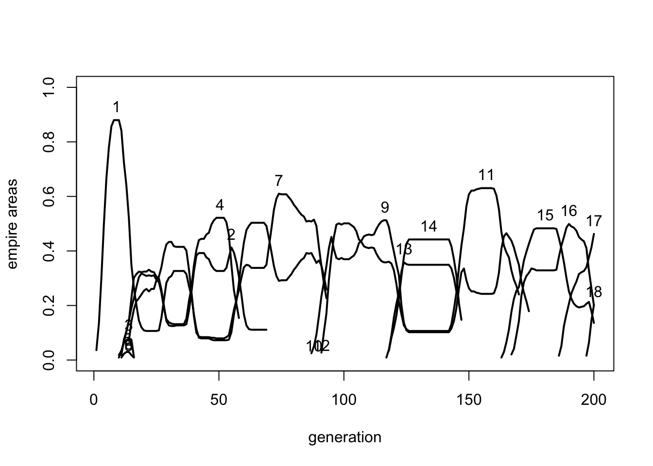
The plot above shows the oscillatory dynamics that we were hoping for, and which resemble real world historical dynamics. No empire dominates the entire time period. Empire 1 soon collapses making way for new empires. Some of these collapse very quickly, others persist for several generations. Even by the final generation here, empires continue to rise and fall, and would continue to do so if we extended the simulation further.
Now let’s systematically remove different elements of the model to see which are necessary for generating these dynamics.
First we manipulate \(h\), the constant which determines how quickly power declines with distance from the empire centre. As \(h\) increases, this distance penalty gets smaller.
Here we reduce \(h\) from the default of \(h = 2\) to \(h = 1\):
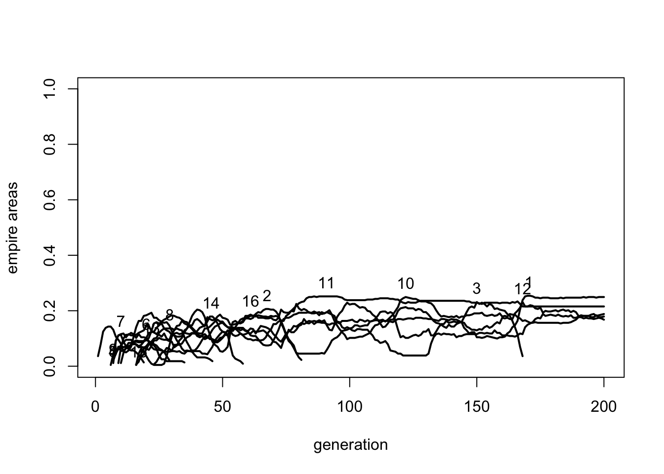
Reducing \(h\) reduces and homogenises the area of each empire. The largest empire barely reaches a third of the total grid, and all empires have roughly the same area. Reducing \(h\) increases the distance penalty in the power equation above. Empires are therefore less able to expand to large sizes, resulting in several smaller empires of roughly equal power continually exchanging frontier groups. While still featuring oscillatory cycles, the lack of large empires and the homogenous empire sizes are not very realistic.
Now we increase \(h\) to 3:
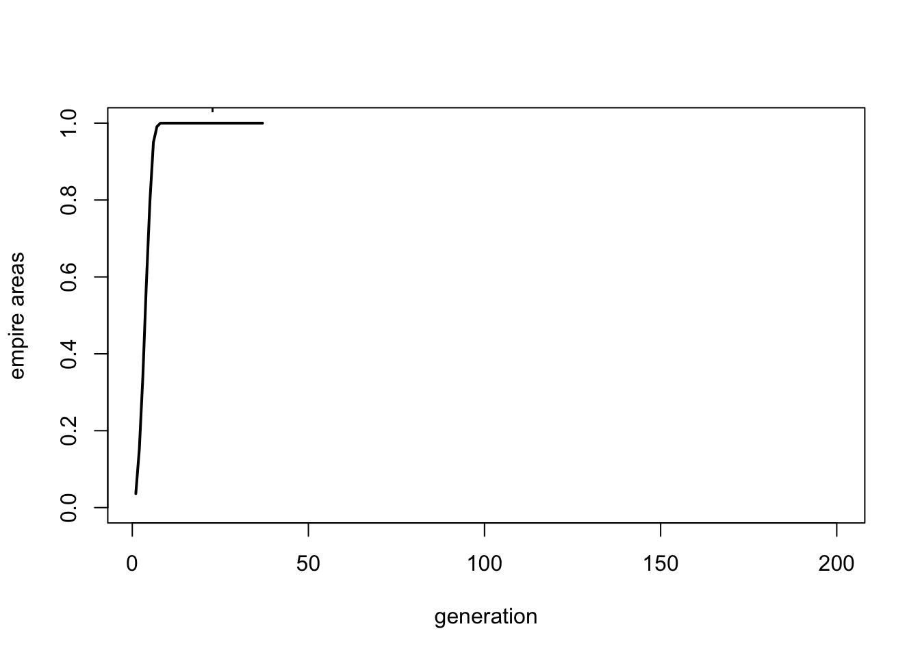
Here Empire 1 quickly fills the entire grid. The lack of any frontier regions means that asabiya then declines until it reaches \(S_{crit}\), at which point it collapses. All groups become nonempire groups, and the lack of any frontiers means that no new empires emerge.
Varying \(h\) therefore indicates that the penalty to large empires of their frontier regions being far from the imperial centre is crucial in generating the oscillatory dynamics representative of real world empires. Too low and empires remain too small, too high and no empires persist at all.
Next we remove the changes in asabiya due to being a frontier or nonfrontier group. Setting \(r_0 = 0\) and \(\delta = 0\) does this.
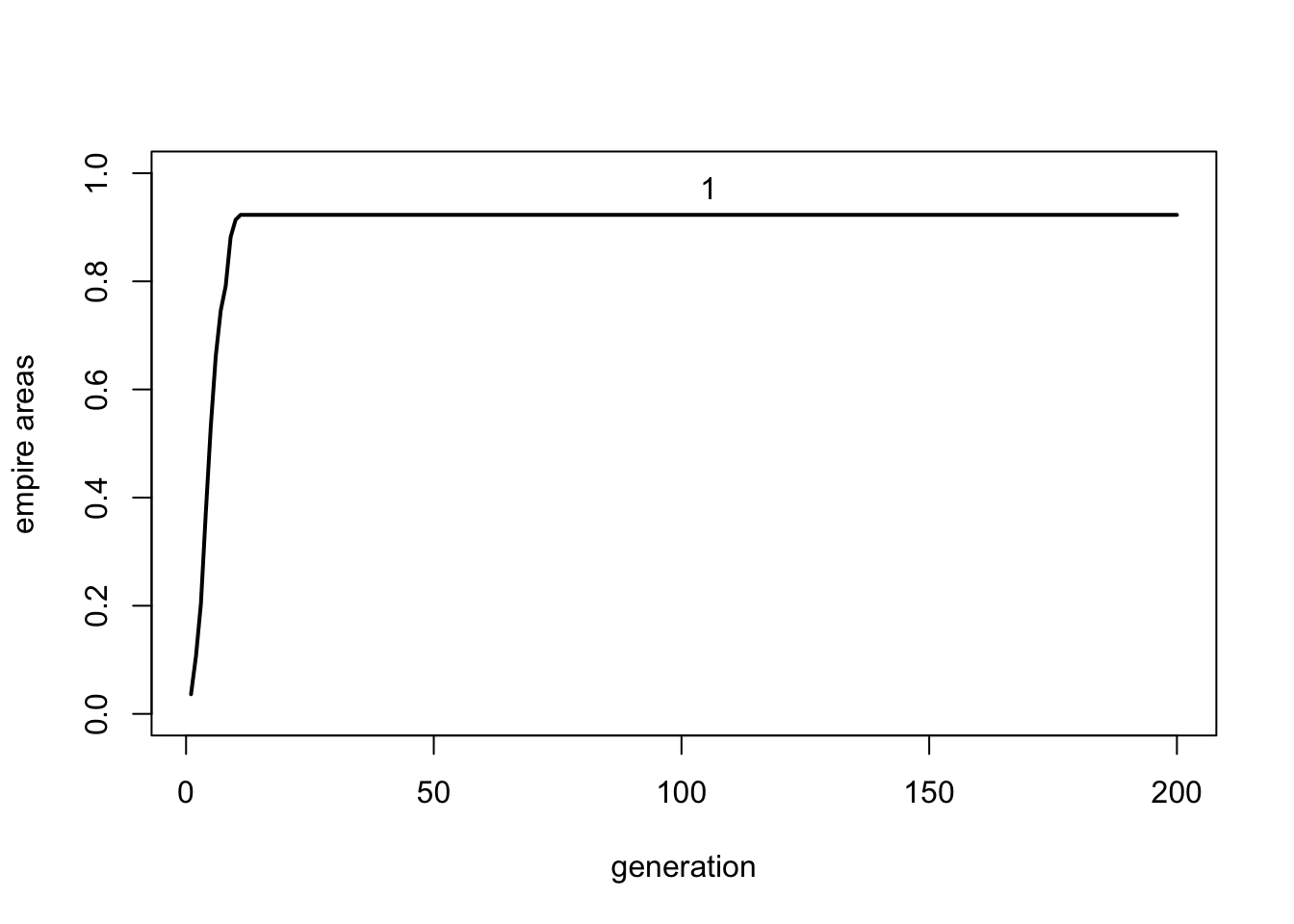
Without frontier-related asabiya changes, the simulation reaches an equilibrium. Empire 1 increases to around 92% of the grid and stays that size. No new empires emerge. This occurs when Empire 1 is large enough such that the power of attackers and defenders (empire and nonempire groups) is equal. This equilibrium behaviour is not a realistic historical dynamic, and indicates that frontier-related changes in asabiya are crucial for generating oscillatory cycles.
Finally we can remove intergroup conflict by setting \(\delta_P\) to a very large number. This means that the inequality \(P_{att} - P_{def} > \delta_P\) is never satisfied, and groups never attack or conquer each other.
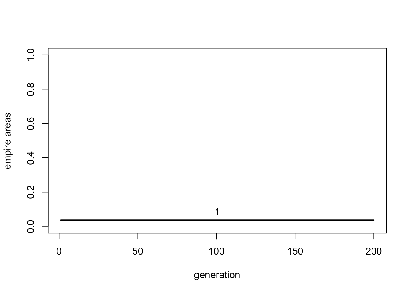
Without intergroup conflict, Empire 1 stays at size 16 for the entire simulation run. No expansion can occur, nor collapse, because groups cannot invade each other. Again, this equilibrium behaviour is historically unrealistic.
Summary
Model 12 simulated the rise and fall of empires throughout human history, recreating an agent-based model presented by Turchin (2003) which tests Turchin’s cultural evolutionary theory of historical dynamics. This theory posits that empires emerge in frontier regions where different ethnic groups exist in close proximity. Such frontier regions are high in asabiya, a form of within-group cooperation. Asabiya provides an advantage in intergroup conflict. Empires emerge when frontier groups high in asabiya conquer neighbouring groups. As these multi-group empires grow larger, they gain power from their larger area and expand further. Large size, however, also reduces the empire’s asabiya as the internal nonfrontier region grows larger. Large size also introduces distance penalties as frontier regions get more distant from the imperial centre of the empire. This weakens the empire, allowing new frontier groups high in asabiya to invade. These invaders become new empires, which expand, then weaken, and the cycle continues.
Model 12 simulated this theory with several assumptions about how the processes above work. We showed that when all processes are operating, then realistic oscillatory dynamics emerge with empires rising and falling continually over the simulation run. When one or more of these processes is removed - specifically, when we remove distance penalties of large empires, changes in asabiya due to being on a frontier, or intergroup conflict - then the dynamics disappear. Instead we see a lack of empires, or a single empire reaching equilibrium size. This lends support to Turchin’s theory linking empire size, asabiya, frontier regions, and power in intergroup conflict.
As Turchin (2003) himself points out (p.71), however, we should be wary of accepting that a theory is correct just because it generates realistic dynamics. Those dynamics may be consistent with many other theories comprising different processes. However, Turchin goes on to test some of the predictions of the model. He shows, for example, that European empires from the years 0 - 1900 almost always emerge in frontier regions, consistent with the model. This lends empirical support to Turchin’s theory, and shows how models can guide empirical research.
There are several ‘black-boxed’ assumptions in the model. For example, why does asabiya decline inside empires? Elsewhere, Turchin (2016) attributes this decline in cooperation to elite overproduction. When there are too many members of ruling elite classes (e.g. politicians, lawyers or scholars), these elites start competing amongst themselves for positions of power rather than working together for the society. This is not modelled here, but a more explicit multi-level selection model might capture this decline in group-level cooperation as a result of greater individual-level competition.
In subsequent work, Turchin et al. (2013) extended the spatially explicit model recreated here from an abstract \(N_{side}\) x \(N_{side}\) grid to a realistic map of Eurasia, and added mechanisms such as the diffusion of military technology that aids in intergroup conflict. This more geographically explicit model recreated specific historical patterns of empire dynamics in the region. Like Model 12, cultural group selection in the form of intergroup conflict, powered by within-group cooperation / asabiya, is crucial for these historical dynamics.
Unlike traditional historians, Turchin (2003) presents both analytic and agent-based models of his verbal theory of historical dynamics. While historians are typically sceptical of formal models, Turchin (2008) has argued for their value in allowing us to precisely state verbal historical explanations, test their internal logic and population-level dynamics in a way that the human brain is ill-equipped for, and provide specific quantitative predictions to then test with historical data. He calls this quantitative science of history ‘cliodynamics’, which can be seen as a branch of cultural evolution. In much of this work, Turchin has drawn on methods and concepts from population ecology (his former discipline). Formal models have been enormously useful in ecology, where population dynamics are often similarly complex yet can be usefully described by simple models. For example, the oscillatory cycles observed in Model 12 are similar to oscillatory predator-prey cycles observed for species such as lynxes and hares, as described by the famous Lotka-Volterra equations.
In terms of programming techniques, we drew here on the spatially-explicit methods of Model 10 (Polarisation). We use multiple matrices to store the empire and asabiya of each group in each cell of the square grid. Unlike previous models, Model 12 features quite a few equations. We have equations describing the increase and decline of asabiya, and equations for calculating the power of each group. While equations are more commonly seen in analytic models than agent-based simulations, we should not be afraid to use them in the latter. The more precise the relations are between different variables, the more straightforward will be our predictions. We can also choose specific functions (e.g. exponential, logistic) which have known properties (e.g. limitless growth vs reaching equilibrium) and may be appropriate to specific situations.
Exercises
Extend the number of timesteps to \(t_{max} = 10000\), or some other large number. Do the same oscillatory dynamics persist or does the simulation ever reach equilibrium?
Vary the grid size via \(N_{side}\), making it both smaller and larger than the default \(N_{side} = 21\). What effect does this have on the dynamics of the model? What implications might we draw for how geography (e.g. small islands vs large continents) affects empire formation?
Modify the initial conditions of the model. What happens if Empire 1 is initially larger or smaller than 16 groups in size? What if there is more than one empire existing at the start?
Modify EmpireDynamics to generate a snapshot of the grid showing the empire id of each cell, similar to the PolarizationPlot and PolarizationMultiplot functions in Model 10 (Polarisation). Use numbers, different symbols or different colors to indicate different empires on the grid. Use these visualisations to test what Turchin (2003) calls the ‘reflux effect’. This is where new empires that emerge at a border with an existing empire tend to expand initially backwards, into the nonempire region, rather than continuing to expand into the existing empire. This is because the existing empire is still quite strong due to its large size. Recreate Turchin’s Fig 4.5 to illustrate the reflux effect.
Frontiers in Model 12 are one group wide and use a von Neumann neighbourhood. That is, a group’s asabiya only increases if at least one of its four NSEW neighbours has a dissimilar empire id. Change this to (i) a Moore neighbourhood, so that asabiya increases if at least one of the eight surrounding groups (including diagonals) have a dissimilar empire id, and (ii) make frontiers \(n_f > 1\) groups wide, such that asabiya increases if at least one group in a \(n_f\)-group radius has a dissimilar empire id (currently \(n_f = 1\)). How do these extended frontiers affect the dynamics? Do these effects make sense given the assumptions of the model?
References
Turchin, P. (2003). Historical dynamics. Princeton University Press.
Turchin, P. (2008). Arise’cliodynamics’. Nature, 454(7200), 34-35.
Turchin, P. (2016). Ultrasociety: How 10,000 years of war made humans the greatest cooperators on earth. Chaplin, CT: Beresta Books.
Turchin, P., Currie, T. E., Turner, E. A., & Gavrilets, S. (2013). War, space, and the evolution of Old World complex societies. Proceedings of the National Academy of Sciences, 110(41), 16384-16389.