Model 18: The evolution of social learning
Introduction
All the previous models in this series have involved purely cultural evolution. We have tracked the frequencies of different cultural traits and how they change in response to different learning biases (e.g. conformity) and demographic processes (e.g. migration). But we can also step back and ask why the capacities for cultural evolution, such as learning biases like conformity, evolved in the first place. These are models of gene-culture coevolution, assuming that there are genes for things like social learning biases, which emerge and spread as a consequence of the adaptive value of the cultural traits that they allow their bearers to acquire.
The most basic question we can ask is why social learning evolved from the presumably ancestral state of individual (asocial) learning. What are the adaptive costs and benefits of learning from others (social learning), rather than learning directly from the environment (individual learning)? A common answer to this question is that social learning evolves because individual learning is more costly than social learning. This premise makes sense, given that learning directly from the environment intuitively seems more costly than copying others. Trying out various mushrooms you find growing in the woods is surely more risky and less adaptive than eating the same mushrooms as you see your neighbour eating, assuming your neighbour isn’t sick or dead.
Rogers (1988) presented a model addressing this question. This model showed that social learning does indeed evolve when it is less costly than individual learning, with social learners coexisting at equilibrium with individual learners. However, Rogers’ model also showed that at this equilibrium, the mean fitness of the entire population is the same as a population composed entirely of individual learners. This contradicts the common claim that social learning (i.e. culture) is on average adaptive for individuals, populations and species. This contradiction has come to be known as “Rogers’ paradox”. Model 18a will recreate these results, before in Model 18b presenting a ‘solution’ to Rogers’ paradox, i.e. a learning strategy that does increase the average fitness of the population relative to individual learning.
Model 18a: Rogers’ model
Although our aim here is to recreate the findings of Rogers (1988), we will mostly follow the form of a more general version of Rogers’ model presented by Enquist et al. (2007). I first describe the model verbally, then build it step by step, before putting it all inside a function.
We assume two types of agents: individual learners and social learners. Individual learners learn directly from the environment once per generation. The result of individual learning is behaviour that is either ‘correct’ or ‘incorrect’ in the current environment. With probability \(p_i\), an individual learner identifies and adopts the correct behaviour. With probability \(1 - p_i\) their behaviour is incorrect. Individual learning, whatever the outcome, entails a fitness cost of \(c_i\).
Social learners pick an agent from the previous generation at random and copy their behaviour. If the random demonstrator had the correct behaviour in the current environment, the social learner adopts the correct behaviour. If the demonstrator had the incorrect behaviour in the current environment, the social learner adopts the incorrect behaviour. This random copying is the unbiased transmission from way back in Model 1. For simplicity, we assume that social learning is 100% accurate (i.e. \(p_s = 1\) in Enquist et al. 2007). We also assume no cost to social learning (i.e. \(c_s = 0\) in Enquist et al. 2007), so that whenever \(c_i > 0\), individual learning is more costly than social learning consistent with our assumption from above.
To avoid negative fitnesses, we assume that all agents have a baseline fitness of 1. Agents with the correct behaviour after learning receive an additional \(b\) units of fitness. Agents with the incorrect behaviour receive no additional fitness benefit.
With probability \(v\) per generation, the environment changes such that all correct behaviours from the previous generation become incorrect. Environmental change won’t affect individual learners, but it means that social learners can no longer copy the correct behaviour from the previous generation and therefore must be incorrect, whoever they copy.
After all agents have done their learning and fitnesses have been calculated, there is selection and reproduction. For simplicity we assume asexual reproduction. \(N\) new agents are created who inherit their learning strategy (individual or social) from the previous generation. Agents reproduce in proportion to their relative fitness. Agents with above average fitness are more likely to reproduce, while agents with below average fitness are less likely.
Finally there is random mutation of learning strategies in the newly created generation. With probability \(\mu\) per agent, an individual learner flips to a social learner, or vice versa. We start in generation \(t = 1\) with a population entirely composed of individual learners and allow mutation to introduce social learners, reflecting the assumption that individual learning is the ancestral state.
In this model we are interested in changes in the frequency of social learners over time, which we denote \(q_s\). The frequency of individual learners is therefore \(1 - q_s\). We can think of this as genetic change, with genes determining whether an agent learns individually or socially (although see Mesoudi et al. 2016 for an alternative perspective).
The first step, as always, is to define our \(N\) agents. They have a learning type, initially all ‘IL’ standing for ‘Individual Learner’, a behaviour, initially NA, and a fitness, also NA.
N <- 100

# create agents, initially all individual learners
agent <- data.frame(learning = rep("IL", N),
                    behaviour = rep(NA, N),
                    fitness = rep(NA, N))

head(agent)
## learning behaviour fitness
## 1 IL NA NA
## 2 IL NA NA
## 3 IL NA NA
## 4 IL NA NA
## 5 IL NA NA
## 6 IL NA NAWe also define our output dataframe which stores, for each timestep, the frequency of social learners, the mean fitness of social learners, and the mean fitness of individual learners, all initially NA. The frequency of individual learners and the population mean fitness can both be calculated from these values.
t_max <- 500

# keep track of freq of social learners and fitnesses
output <- data.frame(SLfreq = rep(NA, t_max),
                     SLfitness = rep(NA, t_max),
                     ILfitness = rep(NA, t_max))

head(output)
## SLfreq SLfitness ILfitness
## 1 NA NA NA
## 2 NA NA NA
## 3 NA NA NA
## 4 NA NA NA
## 5 NA NA NA
## 6 NA NA NAWe now start the cycle of events occurring in each generation. The first event is individual learning, with \(p_i = 0.5\) such that agents have a 50% chance of discovering the correct behaviour:
p_i <- 0.5

# individual learning
agent$behaviour[agent$learning == "IL"] <- sample(c(1,0),
                                                  sum(agent$learning == "IL"),
                                                  replace = TRUE,
                                                  prob = c(p_i, 1 - p_i))

head(agent)
## learning behaviour fitness
## 1 IL 1 NA
## 2 IL 0 NA
## 3 IL 1 NA
## 4 IL 1 NA
## 5 IL 1 NA
## 6 IL 0 NAHere the ‘correct’ behaviour is denoted with a 1, and ‘incorrect’ behaviour with 0. The behaviour of each individual learner is set using the sample command, drawing a 1 with probability \(p_i\) and a 0 with probability \(1 - p_i\). Because we are using 1s and 0s, we can check that the proportion of correct behaviour amongst our \(N\) individual learners is roughly (but probably not exactly) \(p_i\) by taking its mean:
## [1] 0.49Because there are no social learners, we will skip social learning until the next generation. Instead we get the agents’ fitnesses. We use the ifelse command to give agents with the correct behaviour a fitness of \(1 + b\), i.e. the baseline 1 plus \(b\) for being correct, and agents with the incorrect behaviour a fitness of 1, i.e. just the baseline (remember R treats a 1 as the same as TRUE and 0 as the same as FALSE). We then subtract the fitness cost of individual learning \(c_i\) from the individual learners, in this case all agents.
b <- 1
c_i <- 0.2

# get fitnesses
agent$fitness <- ifelse(agent$behaviour, 1 + b, 1)
agent$fitness[agent$learning == "IL"] <- agent$fitness[agent$learning == "IL"] - c_i

head(agent)
## learning behaviour fitness
## 1 IL 1 1.8
## 2 IL 0 0.8
## 3 IL 1 1.8
## 4 IL 1 1.8
## 5 IL 1 1.8
## 6 IL 0 0.8Correct agents should have a fitness of \(1 + b - c_i = 1.8\) while incorrect agents have fitness \(1 - c_i = 0.8\).
Next we record the frequency of social learners, which right now will be zero; the mean fitness of social learners, which will be NA because there aren’t any; and the mean fitness of individual learners. The latter will be approximately equal to the proportion of correct individual learners multiplied by the fitness of correct individual learners plus the proportion of incorrect individual learners multiplied by the fitness of incorrect individual learners, i.e. \(p_i(1 + b - c_i) + (1 - p_i)(1 - c_i) = 1.3\).
t <- 1

# record frequency and fitnesses
output$SLfreq[t] <- sum(agent$learning == "SL") / N
output$SLfitness[t] <- mean(agent$fitness[agent$learning == "SL"])
output$ILfitness[t] <- mean(agent$fitness[agent$learning == "IL"])

head(output)
## SLfreq SLfitness ILfitness
## 1 0 NaN 1.29
## 2 NA NA NA
## 3 NA NA NA
## 4 NA NA NA
## 5 NA NA NA
## 6 NA NA NANext there is selection and reproduction. Similar to how we calculated relative payoffs in Model 4 (indirect bias), here we calculate relative fitness by dividing each agent’s fitness by the sum of all agents’ fitnesses so that they all add up to one. These are then used in a sample command to pick \(N\) new learning types from the current agent dataframe, weighted by the relative_fitness of each of these agents.
# selection and reproduction
relative_fitness <- agent$fitness / sum(agent$fitness)

agent$learning <- sample(agent$learning,
                         N,
                         prob = relative_fitness,
                         replace = TRUE)
Because we only have individual learners, nothing will change here. But now we introduce social learners via mutation. We set a relatively high mutation rate of \(\mu = 0.1\) for demonstration purposes, meaning on average 10% of our individual learners should mutate into social learners. Similar to Model 2a (unbiased mutation), we store agent in previous_agent so that we are not mutating agents that have already mutated, then get \(N\) TRUE/FALSE values based on \(\mu\), then mutate ILs into SLs and SLs into ILs according to these TRUE/FALSE values.
mu <- 0.1

# mutation
previous_agent <- agent

mutate <- runif(N) < mu

agent$learning[previous_agent$learning == "IL" & mutate] <- "SL"
agent$learning[previous_agent$learning == "SL" & mutate] <- "IL"

sum(agent$learning == "SL")
## [1] 15The number of social learners should be around \(\mu N = 10\).
Now that we have some social learners we can implement social learning, imagining that we’re now in the next generation. In the code below, first we store the current agent dataframe in previous_agent so that social learners can copy the previous generation. In the full code we would do this at the very start of the generation, before individual learning has changed behaviours. Then we check whether the environment has changed by comparing \(v\) against a single random number from 0 to 1 generated with runif. If the environment has changed, then all social learners must by assumption have the incorrect behaviour, irrespective of who they copy. If the environment hasn’t changed, then we store a random selection of demonstrators from previous_agent in dem, and then give the correct behaviour to social learners who have copied a correct demonstrator, and incorrect behaviour to social learners who have copied an incorrect demonstrator (remembering again that because behaviour is stored as a 1 or 0 and R treats these as TRUE and FALSE, dem returns all the correct demonstrators as TRUE and incorrect demonstrators as FALSE, and !dem returns the reverse).
v <- 0.9

# store previous timestep agent
previous_agent <- agent

# social learning

# if environment has changed, all social learners have incorrect beh
if (v < runif(1)) {

  agent$behaviour[agent$learning == "SL"] <- 0 # incorrect

} else {

  # otherwise for each social learner, pick a random demonstrator from previous timestep
  # if demonstrator is correct, adopt correct beh

  dem <- sample(previous_agent$behaviour, N, replace = TRUE)

  agent$behaviour[agent$learning == "SL" & dem] <- 1 # correct
  agent$behaviour[agent$learning == "SL" & !dem] <- 0 # incorrect

}

agent[agent$learning == "SL",1:2]
## learning behaviour
## 2 SL 1
## 5 SL 0
## 10 SL 0
## 15 SL 1
## 18 SL 1
## 19 SL 1
## 36 SL 1
## 48 SL 1
## 52 SL 0
## 55 SL 1
## 58 SL 1
## 69 SL 1
## 77 SL 1
## 89 SL 0
## 90 SL 1Here you should see some social learners have acquired the correct behaviour (1) and some incorrect (0), unless the environment changed in which case they’re all incorrect. Rerun the code to see the different outcomes. Note that I omitted fitness from the displayed dataframe because it will be out of date, as we haven’t re-calculated fitnesses based on these new behaviours.
The following function RogersModel puts all these bits together, with the within-generation events inside a t-loop and some default parameter values in the declaration. We use a larger \(N = 10000\) to reduce stochasticity and better resemble the dynamics of Rogers’ original analytic model, and a lower \(\mu = 0.001\) to prevent mutation from affecting the frequencies too much. Note also that we add a column to the output dataframe to store the predicted fitness of individual learners given the parameter values; this will be used in the plots coming up next.
RogersModel <- function(N=10000, t_max=1000, p_i=0.5, b=1, c_i=0.2, mu=0.001, v=0.9) {

  # create agents, initially all individual learners
  agent <- data.frame(learning = rep("IL", N),
                      behaviour = rep(NA, N),
                      fitness = rep(NA, N))

  # keep track of freq of social learners and fitnesses
  output <- data.frame(SLfreq = rep(NA, t_max),
                       SLfitness = rep(NA, t_max),
                       ILfitness = rep(NA, t_max))

  # start timestep loop
  for (t in 1:t_max) {

    # store previous timestep agent
    previous_agent <- agent

    # individual learning:
    agent$behaviour[agent$learning == "IL"] <- sample(c(1,0),
                                                      sum(agent$learning == "IL"),
                                                      replace = TRUE,
                                                      prob = c(p_i, 1 - p_i))

    # social learning
    # if environment has changed, all social learners have incorrect beh
    if (v < runif(1)) {

      agent$behaviour[agent$learning == "SL"] <- 0 # incorrect

    } else {

      # otherwise for each social learner, pick a random demonstrator from previous timestep
      # if demonstrator is correct, adopt correct beh

      dem <- sample(previous_agent$behaviour, N, replace = TRUE)

      agent$behaviour[agent$learning == "SL" & dem] <- 1 # correct
      agent$behaviour[agent$learning == "SL" & !dem] <- 0 # incorrect

    }

    # get fitnesses
    agent$fitness <- ifelse(agent$behaviour, 1 + b, 1)
    agent$fitness[agent$learning == "IL"] <- agent$fitness[agent$learning == "IL"] - c_i

    # record frequency and fitnesses
    output$SLfreq[t] <- sum(agent$learning == "SL") / N
    output$SLfitness[t] <- mean(agent$fitness[agent$learning == "SL"])
    output$ILfitness[t] <- mean(agent$fitness[agent$learning == "IL"])

    # selection and reproduction
    relative_fitness <- agent$fitness / sum(agent$fitness)

    agent$learning <- sample(agent$learning,
                             N,
                             prob = relative_fitness,
                             replace = TRUE)

    # mutation
    previous_agent <- agent
    mutate <- runif(N) < mu

    agent$learning[previous_agent$learning == "IL" & mutate] <- "SL"
    agent$learning[previous_agent$learning == "SL" & mutate] <- "IL"

  }

  # add predicted IL fitness to output and export
  output$predictedILfitness <- 1 + b*p_i - c_i
  output

}
We also define a plotting function RogersPlots to plot the proportion of social learners over time and the mean fitnesses of each type of learner, plus the mean population fitness, all obtained from the output generated by RogersModel. Note the use of the rgb() command with the argument alpha for the fitness colors. This generates transparent lines so that we can still see them all when they overlap, which they often will.
RogersPlots <- function(output) {

  par(mfrow=c(1,2)) # 1 row, 2 columns

  plot(output$SLfreq,
       type = 'l',
       lwd = 2,
       ylim = c(0,1),
       ylab = "proportion of social learners",
       xlab = "generation")

  # calculate population mean fitness
  POPfitness <- output$SLfreq * output$SLfitness + (1 - output$SLfreq) * output$ILfitness

  alpha=150
  plot(output$SLfitness,
       type = 'l',
       lwd = 2,
       col = rgb(255,165,0,max=255,alpha), # orange
       ylim = c(0.5,2),
       ylab = "mean fitness",
       xlab = "generation")
  lines(output$ILfitness,
        type = 'l',
        lwd = 2,
        col = rgb(65,105,225,max=255,alpha)) # royalblue
  lines(POPfitness,
        type = 'l',
        lwd = 2,
        col = rgb(100,100,100,max=255,alpha)) # grey
  abline(h = output$predictedILfitness[1],
         lty = 2,
         lwd = 2)
  legend("bottom",
       legend = c("social learners", "individual learners", "population"),
       col = c(rgb(255,165,0,max=255,alpha),
               rgb(65,105,225,max=255,alpha),
               rgb(100,100,100,max=255,alpha)),
       lty = 1,
       lwd = 2,
       bty = "n",
       cex = 0.9)

}
Here’s one run of RogersModel with default parameter values:
We can see that there is a majority of social learners, fluctuating around a proportion of 0.8. There is quite a bit of fluctuation though. There is also fluctuation in the mean fitness of social learners, and consequently the mean population fitness, although the mean fitness of individual learners is fairly constant. The black dotted line shows the predicted mean fitness of individual learners, i.e. \(1 + bp_i - c_i\). The blue individual learner line from the simulations matches this value quite well, barring small fluctuations because \(p_i\) is a probability rather than deterministic.
Note also that the mean fitness of social learners and the whole population also fluctuate around this value: sometimes higher, but often lower. This is Rogers’ paradox. Even though we have a majority of social learners, the mean population fitness does not on average exceed the fitness of individual learners.
The reason for the fluctuations is environmental change. When the environment changes, all behaviour in the previous generation becomes incorrect. Social learners therefore copy incorrect behaviour, and are at a disadvantage compared to individual learners for whom environmental change is irrelevant. Individual learners always ignore the previous generation and sample directly from the current environment. However, once at least some individual learners have discovered the correct behaviour, social learners then have the upper hand due to the lower costs of social learning compared to individual learning. Social learners can copy the correct behaviour from the previous generation at no cost, whereas individual learners always pay a cost \(c_i\) for accuracy \(p_i\). Social learners therefore increase in frequency, replacing individual learners. And the longer the environment remains constant, the more correct social learners there will be for new social learners to copy. That is, until the environment changes again, at which point the individual learners regain the advantage. And so on. The fluctuations in the left hand plot above are caused by this cycling back and forth between individual and social learners having the advantage.
At equilibrium, the fitness of individual and social learners must by definition be equal. Because individual learners’ fitness is fixed at \(1 + bp_i - c_i\), then the mean fitness of social learners must also be this value. Hence Rogers’ paradox: the mean fitness of the population with social learners is no greater than that of a population entirely composed of individual learners. Culture makes no difference. The analytical appendix confirms this, and contains equations for calculating the equilibrium proportion of social learners for a given set of parameter values.
We can check this argument by manipulating our parameters. If we remove environmental change by setting \(v = 1\), then according to the above logic, social learners should entirely replace individual learners. This is because social learners will acquire the correct behaviour from individual learners at the start, replace individual learners because they do not pay the cost of individual learning, and never suffer from their behaviour becoming out of date because the environment never changes.
This is indeed what happens: the proportion of social learners goes almost to fixation, barring individual learners introduced each generation by mutation, and the mean fitness of social learners (and by extension the population, which is almost all social learners) clearly exceeds that of individual learners. The paradox is solved, in a way - if we are happy to assume that environments never change.
We can also check that the cost of individual learning is providing the advantage to social learners. Let’s reduce this cost to \(c_i = 0.1\), reintroducing the default value of environmental change:
As predicted, the proportion of social learners has dropped to around 0.5. Because environmental change is back, Rogers’ paradox is also restored.
Model 18b: Critical social learning
Rogers’ model shows that social learning can evolve when it is less costly than individual learning, but that it does not increase the mean population fitness, contrary to claims that culture is adaptive. One solution to this ‘paradox’ is removing environmental change. However, this seems unrealistic as environments are always changing in some way.
Another solution to Rogers’ paradox is to relax the unrealistic assumption that agents can either only learn individually or only learn socially. Obviously real organisms can do both. The evolution of social learning did not replace individual learning, it supplemented it. Indeed, social learning may rely on the same associative learning mechanisms as individual learning (Heyes 2012).
Enquist et al. (2007) therefore proposed a third, more plausible strategy: a critical social learner. These critical social learners learn socially first, and if the copied solution is incorrect, they then learn individually. Model 18b adds critical social learners to the simulation to see whether they do better than pure social and pure individual learners, and whether they overcome Rogers’ paradox.
The following function EnquistModel adapts RogersModel to include critical learners. The parameters and their defaults are identical, as is the agent dataframe. The output dataframe now tracks the frequency and mean fitness of critical learners (“CL”s) in addition to social and individual learners. Individual learners individually learn as before, then both social and critical learners socially learn. The major new block of code implements individual learning for the incorrect critical learners. However, the actual code and fitness assignments are identical to those earlier in the function for individual learners, so there’s nothing new here. The final difference is mutation, which now includes critical learners.
EnquistModel <- function(N=10000, t_max=500, p_i=0.5, b=1, c_i=0.2, mu=0.001, v=0.9) {

  # create agents, initially all individual learners
  agent <- data.frame(learning = rep("IL", N),
                      behaviour = rep(NA, N),
                      fitness = rep(NA, N))

  # track the proportion and mean fitness of each learning type
  output <- data.frame(SLfreq = rep(NA, t_max),
                       ILfreq = rep(NA, t_max),
                       CLfreq = rep(NA, t_max),
                       SLfitness = rep(NA, t_max),
                       ILfitness = rep(NA, t_max),
                       CLfitness = rep(NA, t_max))

  # start timestep loop
  for (t in 1:t_max) {

    # store previous timestep agent
    previous_agent <- agent

    # individual learning:
    agent$behaviour[agent$learning == "IL"] <- sample(c(1,0),
                                                      sum(agent$learning == "IL"),
                                                      replace = TRUE,
                                                      prob = c(p_i, 1 - p_i))

    # social learning for social and critical learners

    # if environment has changed, all social/critical learners have incorrect beh
    if (v < runif(1)) {

      agent$behaviour[agent$learning != "IL"] <- 0 # incorrect

    } else {

      # otherwise for each social learner, pick a random demonstrator from previous timestep
      # if demonstrator is correct, adopt correct beh

      dem <- sample(previous_agent$behaviour, N, replace = TRUE)

      agent$behaviour[agent$learning != "IL" & dem] <- 1 # correct
      agent$behaviour[agent$learning != "IL" & !dem] <- 0 # incorrect

    }

    # get fitnesses
    agent$fitness <- ifelse(agent$behaviour, 1 + b, 1)
    agent$fitness[agent$learning == "IL"] <- agent$fitness[agent$learning == "IL"] - c_i

    # incorrect critical learners engage in individual learning
    CL_0 <- agent$learning == "CL" & agent$behaviour == 0

    agent$behaviour[CL_0] <- sample(c(1,0),
                                    sum(CL_0),
                                    replace = TRUE,
                                    prob = c(p_i, 1-p_i))

    agent$fitness[CL_0 & agent$behaviour] <- agent$fitness[CL_0 & agent$behaviour] + b
    agent$fitness[CL_0] <- agent$fitness[CL_0] - c_i

    # record frequency and fitnesses before reproduction and mutation
    output$SLfreq[t] <- sum(agent$learning == "SL") / N
    output$ILfreq[t] <- sum(agent$learning == "IL") / N
    output$CLfreq[t] <- sum(agent$learning == "CL") / N
    output$SLfitness[t] <- mean(agent$fitness[agent$learning == "SL"])
    output$ILfitness[t] <- mean(agent$fitness[agent$learning == "IL"])
    output$CLfitness[t] <- mean(agent$fitness[agent$learning == "CL"])

    # selection and reproduction
    relative_fitness <- agent$fitness / sum(agent$fitness)

    agent$learning <- sample(agent$learning,
                             N,
                             prob = relative_fitness,
                             replace = TRUE)

    # mutation
    mutate <- runif(N) < mu
    IL_mutate <- agent$learning == "IL" & mutate
    SL_mutate <- agent$learning == "SL" & mutate
    CL_mutate <- agent$learning == "CL" & mutate

    agent$learning[IL_mutate] <- sample(c("SL","CL"),
                                        sum(IL_mutate),
                                        replace = TRUE)

    agent$learning[SL_mutate] <- sample(c("IL","CL"),
                                        sum(SL_mutate),
                                        replace = TRUE)

    agent$learning[CL_mutate] <- sample(c("SL","IL"),
                                        sum(CL_mutate),
                                        replace = TRUE)

  }

  # add predicted IL fitness to output and export
  output$predictedILfitness <- 1 + b*p_i - c_i
  output

}
And here is a new plotting function for EnquistModel, plotting the frequency and mean fitness of CLs:
EnquistPlots <- function(output) {

  par(mfrow=c(1,2)) # 1 row, 2 columns

  # plot frequencies
  plot(output$SLfreq,
       type = 'l',
       lwd = 2,
       col = "orange",
       ylim = c(0,1),
       ylab = "proportion of social learners",
       xlab = "generation")
  lines(output$ILfreq,
        type = 'l',
        lwd = 2,
        col = "royalblue")
  lines(output$CLfreq,
        type = 'l',
        lwd = 2,
        col = "springgreen4")
  legend(x = nrow(output)/10, y = 0.6,
         legend = c("social learners", "individual learners", "critical learners"),
         col = c("orange", "royalblue", "springgreen4"),
         lty = 1,
         lwd = 2,
         bty = "n",
         cex = 0.8)

  alpha=150

  plot(output$SLfitness,
       type = 'l',
       lwd = 2,
       col = rgb(255,165,0,max=255,alpha), # orange
       ylim = c(0.5,2),
       ylab = "mean fitness",
       xlab = "generation")
  lines(output$ILfitness,
        type = 'l',
        lwd = 2,
        col = rgb(65,105,225,max=255,alpha)) # royalblue
  lines(output$CLfitness,
        type = 'l',
        lwd = 2,
        col = rgb(0,139,69,max=255,alpha)) # springgreen4
  abline(h = output$predictedILfitness[1],
         lty = 2)
  legend("bottom",
       legend = c("social learners", "individual learners", "critical learners"),
       col = c(rgb(255,165,0,max=255,alpha),
               rgb(65,105,225,max=255,alpha),
               rgb(0,139,69,max=255,alpha)),
       lty = 1,
       lwd = 2,
       bty = "n",
       cex = 0.8)

}
We can now run EnquistModel with default parameter values:
The left hand plot clearly shows that critical learners almost dominate the population, barring the occasional other types introduced each generation by mutation. The right hand plot shows why: the fitness of individual learners hovers around the expected value shown by the dotted line, the fitness of social learners fluctuates both above and below the dotted line depending on whether the environment has changed recently, while the fitness of critical learners also fluctuates but never drops below the dotted line. Critical learners have the best of both worlds: they can copy previous solutions at lower cost than individual learning when the environment is stable, but when the environment changes, they can detect that change and discover the new correct behaviour.
Summary
Rogers’ model, and even Enquist et al’s extension, are hugely unrealistic in many ways. Despite this, these models give valuable insights into the evolutionary advantages and disadvantages of social learning relative to individual learning. Social learning benefits from being less costly than individual learning. Yet social learning does not respond well to environmental change. When environments change, social learners are left copying each other’s outdated incorrect behaviour. Individual learners suffer no such penalty when the environment changes. This trade off can lead to a mixed equilibrium where individual and social learners coexist.
Rogers’ model resembles producer-scrounger models from ecology (Barnard & Sibly 1992). In a feeding context, ‘producer’ birds discover new sources of food, while ‘scrounger’ birds follow the producers and exploit the food sources they find. In Rogers’ model, individual learners are ‘information producers’ discovering new cultural traits, while social learners are ‘information scroungers’ copying the producers’ cultural traits without paying the cost.
In a feeding context it seems fairly obvious that scroungers do not contribute anything to the overall mean fitness of the group, population or species. Yet it wasn’t until Rogers’ model that the same was recognised for social learning. Mixed populations of social and individual learners have no greater mean fitness than populations entirely composed of individual learners. This came to be known as Rogers’ Paradox, given that social learning and culture are often thought of as the secret of our species’ evolutionary success. In Rogers’ model, this is wrong.
However, models are only as good as their assumptions, and one major assumption of Rogers’ model is that individuals can perform only one of the two kinds of learning. Real organisms do both. Hence Enquist et al. (2007), recreated here in Model 18b, showed that a ‘critical learner’ strategy of first learning socially and, if this results in incorrect behaviour, then engaging in individual learning, outperforms and replaces both pure individual learning and pure social learning. This might seem obvious in hindsight but was not fully recognised until Rogers’ simple model and its extensions.
We should therefore expect cultural species to be composed of individuals who mostly learn socially early in life, then supplement this with individual learning later on. This seems to be the pattern in humans, where children are powerful, almost compulsive imitators (Lyons et al. 2007), while adolescents and adults do more experimentation and try to improve what they’ve learned during childhood.
Critical social learning can also be seen as supporting a form of cumulative culture. As critical learners increase in frequency, each new generation contains more and more correct individuals. New critical learners can copy these accumulated correct behaviours for free. That is, until the environment changes, at which point the accumulation begins again.
Enquist et al.’s model is still extremely simple. Real populations learn and accumulate multiple traits, not just one. Environmental change rarely causes all knowledge to be wiped out requiring cultural evolution to start from scratch. Organisms have more complex developmental ‘learning schedules’, undergoing multiple bouts of social and individual learning during their lifetimes. And there is no spatial or social structure in these models. Recent work has addressed some of these limitations (e.g. Rendell et al. 2010; Lehmann et al. 2013), but others remain to be modelled, and all require further empirical testing.
In terms of modelling techniques, Model 18 showed how to model the evolution of a capacity for cultural evolution, rather than just the cultural evolution of a socially learned trait. We specified the fitness costs and benefits of each learning strategy under different conditions, implemented selection and reproduction based on differential fitness, as well as the mutation of strategies. We then see which learning strategy, or mix of strategies, constitute an evolutionarily stable strategy after multiple generations for a given set of parameters. If we assume that the learning strategy is genetically specified, then this is a gene-culture coevolution model, where genetic strategies and cultural traits coevolve. The analytic appendix below shows how to derive the exact evolutionarily stable mix of strategies for specific parameter values, confirming and clarifying our simulation results.
Exercises
In RogersModel, what should happen to the proportion of social learners and the mean fitnesses when \(v=0\), i.e. the environment changes every generation? Run the simulation to check your predictions.
Add a cost to social learning, \(c_s\), and an accuracy of social learning, \(p_s\), to RogersModel. What effect do these variables have on the dynamics of the model?
Add multiple runs to both RogersModel and EnquistModel, and plot the mean frequencies and fitnesses across all \(r_{max}\) runs. Does this show Rogers’ paradox as clearly as just plotting one run, as shown above?
Enquist et al. (2007) also modelled a ‘conditional social learner’ who learns individually first and if incorrect learns socially - the reverse of critical social learners. Add conditional social learners to EnquistModel. How do conditional learners fare against critical learners and individual learners?
Analytical Appendix
We start with Model 18a, containing just individual and social learners. Following Enquist et al. (2007) we can derive expressions for the equilibrium frequency of social learning, and the fitnesses of social and individual learning. Note that we omit their \(c_s\) and \(p_s\) for simplicity, and to match the simulations above.
As already specified above, the fitness of individual learners, \(w_i\), is given by:
\[ w_i = 1 + bp_i - c_i \hspace{30 mm}(18.1)\]
where the benefit \(b\) of correct behaviour is received with probability \(p_i\), minus the cost of individual learning \(c_i\).
For social learners, the benefit \(b\) is received when (i) a correct demonstrator from the previous generation is copied, with probability equal to the proportion of correct behaviour amongst all agents in the previous generation, denoted \(q_{t-1}\), as long as (ii) the environment remains the same, which happens with probability \(v\). The fitness of social learners, \(w_s\), is therefore:
\[ w_s = 1 + bq_{t-1}v \hspace{30 mm}(18.2)\]
If \(q_i\) and \(q_s\) are the proportions of individual and social learners respectively in generation \(t\), then the frequency of correct behaviour in generation \(t\), \(q_t\), is given by:
\[ q_t = q_i p_i + q_s q_{t-1} v \hspace{30 mm}(18.3)\]
At equilibrium, \(q_t = q_{t-1} = q^*\), and we know that \(q_i = 1 - q_s\), so:
\[ q^* = (1 - q_s) p_i + q_s q^* v \hspace{30 mm}(18.4)\]
Rearranging Equation 18.4 gives:
\[ q^* = \frac{(1 - q_s) p_i}{1 - q_s v} \hspace{30 mm}(18.5)\]
Replacing \(q_{t-1}\) in Eq 18.2 with \(q^*\) gives:
\[ w_s = 1 + \frac{(1 - q_s) b p_i v}{1 - q_s v} \hspace{30 mm}(18.6)\]
At equilibrium we also know that \(w_i = w_s\). Setting 18.1 equal to 18.6 and rearranging for \(q_s\) gives the frequency of social learners at equilibrium:
\[ q^*_s = \frac{c_i - bp_i(1-v)}{c_i v} \hspace{30 mm}(18.7)\]
For the default parameter values of RogersModel, \(q^*_s\) is
## [1] 0.8333333which is roughly the proportion found in the simulation (although given the fluctuations it’s difficult to tell, which is one advantage of analytical models over simulations).
The next simulation used \(v = 1\). From Equation 18.7 we can see that \(v = 1\) always yields \(q^*_s = c_i / c_i = 1\), i.e. 100% social learners, as found in the simulation (barring mutation, which is not included in the analytical model).
Finally we simulated \(c_i = 0.1\), which gives:
## [1] 0.5555556which again matches the final simulation plot showing that roughly half the agents are social learners (again, with lots of fluctuation).
We can use Equations 18.1 and 18.6 to create a plot that encapsulates Rogers’ paradox, showing the mean fitness of individual learners, social learners, and the entire population as a function of the proportion of social learners, \(q_s\).
# parameter values
p_i <- 0.5
b <- 1
c_i <- 0.1
v <- 0.9

# x-axis, frequency of social learners, q_s
q_s <- seq(0, 1, 0.01)

# fitness of ILers, w_i (Eq 18.1)
w_i <- 1 + b*p_i - c_i

# fitness of SLers, w_s (Eq 18.6)
w_s <- 1 + ((1 - q_s)*b*p_i*v)/ (1 - q_s*v)

# mean population fitness
w <- w_s*q_s + w_i*(1 - q_s)

plot(x = q_s,
     y = w_s,
     type = 'l',
     lwd = 2,
     xlab = "proportion of social learners",
     ylab = "fitness",
     ylim = c(1,1.5),
     lty = 3)
abline(h = w_i,
       lty = 2,
       lwd = 2)
lines(x = q_s,
      y = w,
      lty = 1,
      lwd = 2)
legend(x = 0,
       y = 1.2,
       legend = c("individual learner", "social learner", "population"),
       lty = c(2, 3, 1),
       bty = "n",
       lwd = 2)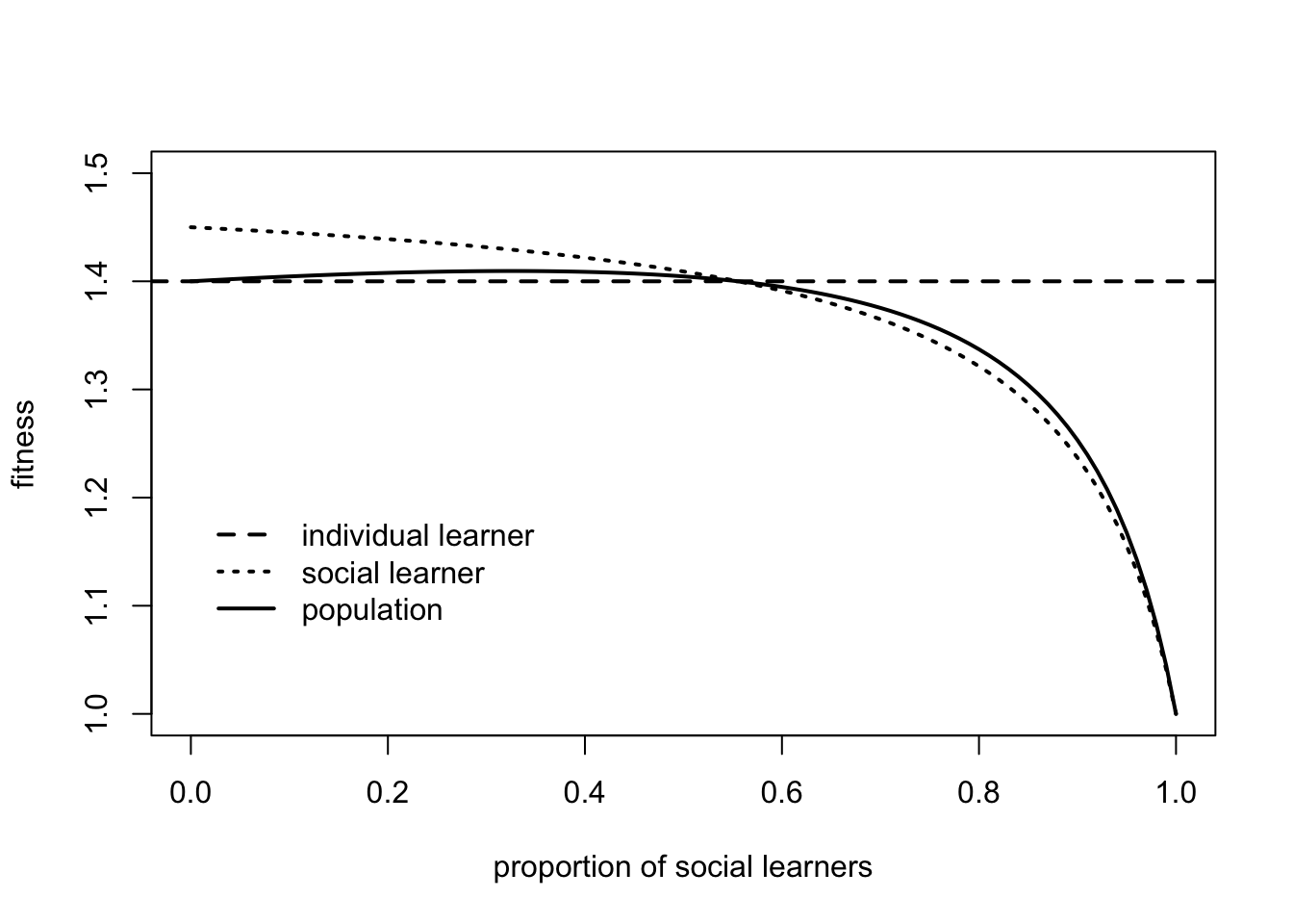
This qualitatively recreates Fig 1 in Rogers (1988) and Fig 1b in Enquist et al. (2007). The point where the three lines cross is the equilibrium frequency of social learners, \(q^*\), from above, where the fitness of individual learners and social learners is equal.
The figure above shows that the fitness of individual learners does not change with the proportion of social learners. It depends on the fixed parameters \(b\), \(p_i\) and \(c_i\). The fitness of social learners, however, does change, with social learners doing well when relatively uncommon (\(q_s < q^*\)), and poorly when common (\(q_s > q^*\)). We can say that the fitness of social learners is frequency-dependent, i.e. its fitness depends at least partly on its own frequency in the population.
As noted above, the underlying reason for this frequency dependence is the balance between environmental change favouring individual learning and costly individual learning favouring social learning. At the extreme left of the graph, when \(q_s = 0\), a single social learner will have fitness \(w_s = 1 + b p_i v\), compared to \(w_i = 1 + b p_i - c_i\). Hence the social learner will get the benefit \(b\) of copying the correct behaviour from the previous generation of individual learners with probability \(p_i\), assuming the environment has stayed the same (with probability \(v\)) and without paying the cost \(c_i\). Hence the advantage of social learning is greater when \(v\) and \(c_i\) are both larger. As we move to the right of the plot, increasing numbers of social learners means that social learners will be increasingly copying other social learners. When the environment changes, there will be fewer individual learners to discover the correct behaviour, and social learners will be increasingly disadvantaged. When \(q_s > q^*\), this disadvantage outweighs the benefits of not paying the costs of individual learning, and individual learners do better.
We now add critical social learners. Their fitness, \(w_c\), is given by the fitness of social learners \(w_s\) plus the fitness of individual learners \(w_i\) weighted by the probability that social learners are incorrect, \((1 - v)\):
\[ w_c = w_s + w_i (1 - v) = 1 + bq_{t-1}v + (bp_i - c_i) (1 - v) \hspace{30 mm}(18.8)\]
The proportion of correct behaviour in the current generation \(q_t\), previously given in Eq 18.3, must now contain an additional term for the frequency of correct behaviour amongst critical learners, \(q_c\):
\[ q_t = q_i p_i + q_s q_{t-1} v + q_c (q_{t-1} v + (1 - q_{t-1} v) p_i) \hspace{30 mm}(18.9)\]
Setting \(q_t = q_{t-1} = q^*\) and \(q_i = 1 - q_s - q_c\), after rearranging we get:
\[ q^* = \frac{p_i (1 - q_s)}{(1 - v (q_s + q_c (1 - p_i))} \hspace{30 mm}(18.10)\]
At equilibrium, critical learners must have higher fitness than social learners if individual learning is adaptive (i.e. from Eq 18.8, when \(w_i > 0\), assuming \(v < 1\)). Hence at equilibrium \(q_s = 0\), such that Eq 18.10 simplifies to:
\[ q^* = \frac{p_i }{1 - v q_c (1 - p_i)} \hspace{30 mm}(18.11)\]
Substituting Eq 18.11 into Eq 18.8 with \(q_{t-1} = q^*\) gives:
\[ w_c = 1 + \frac{b v p_i}{1 - v q_c (1 - p_i)} + (bp_i - c_i) (1 - v) \hspace{30 mm}(18.12)\]
This allows us to plot the fitness of critical learners \(w_c\) against the proportion of critical learners \(q_c\), alongside the fixed fitness of individual learners, similar to what we did with social learners in the previous plot:
# parameter values
p_i <- 0.5
b <- 1
c_i <- 0.1
v <- 0.9

# x-axis, frequency of critical learners, q_c
q_c <- seq(0, 1, 0.01)

# fitness of ILers, w_i (Eq 18.1)
w_i <- 1 + b*p_i - c_i

# fitness of CLers, w_s (Eq 18.12)
w_c <- 1 + (b*v*p_i) / (1 - v*q_c*(1 - p_i)) + (b*p_i - c_i)*(1 - v)

plot(x = q_c,
     y = w_c,
     type = 'l',
     lwd = 2,
     xlab = "proportion of critical learners",
     ylab = "fitness",
     ylim = c(1,2),
     lty = 1)
abline(h = w_i,
       lty = 2,
       lwd = 2)
legend(x = 0,
       y = 1.2,
       legend = c("individual learner", "critical learner"),
       lty = c(2, 1),
       bty = "n",
       lwd = 2)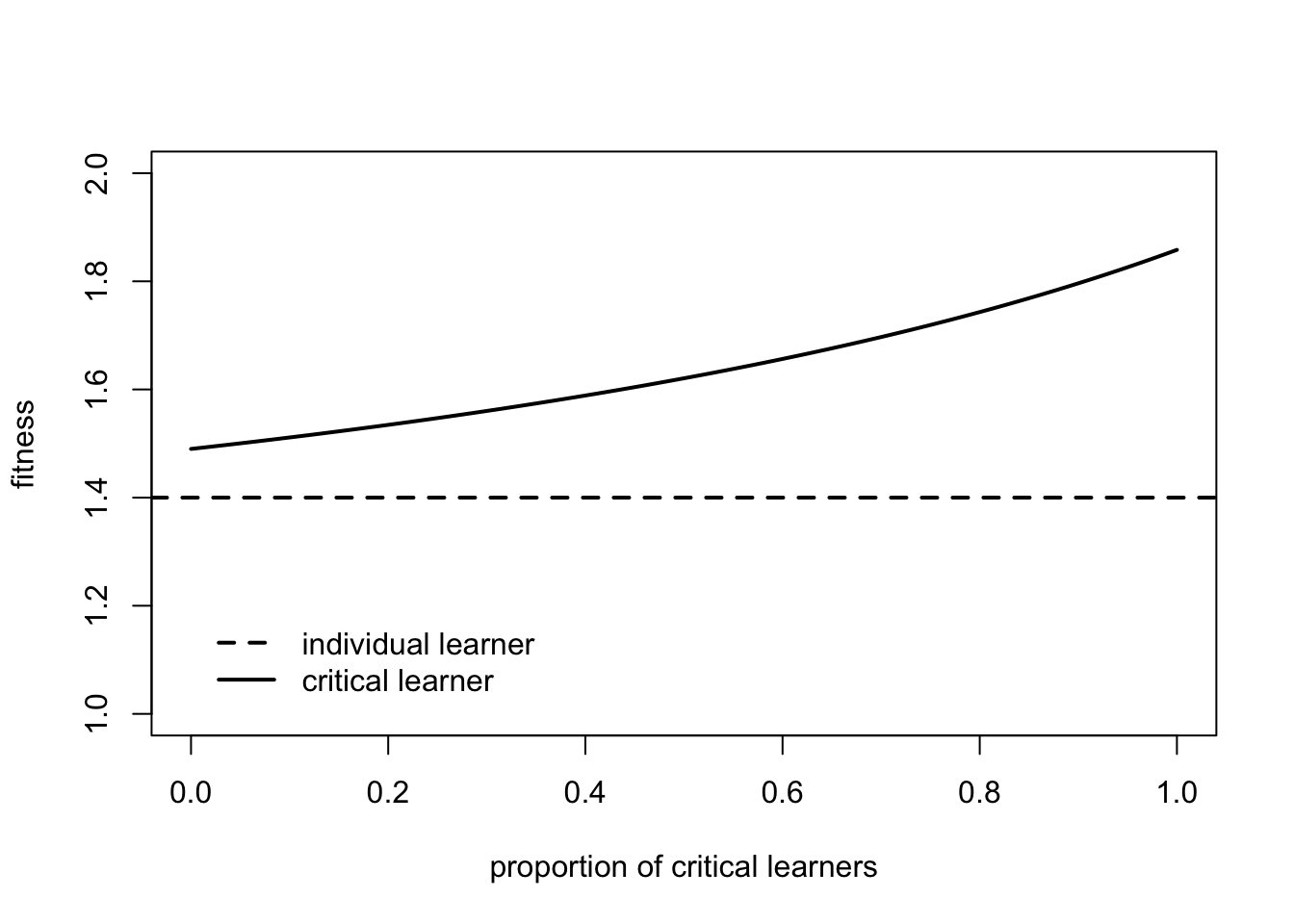
This illustrates the evolutionary advantage of critical learners. Whereas the fitness of social learners decreased with their frequency, the fitness of critical learners increases with their frequency, and is always greater than that of individual learners.
This is again due to the combined action of environmental change and costly individual learning. At the extreme left, when \(q_c = 0\), Eq 18.12 tells us that a single critical learner will have fitness \(w_c = 1 + bp_i - c_i (1 - v)\). This is identical to the fitness of individual learners except the final term \(c_i\) is multiplied by \((1 - v)\), the probability of the environment changing. This reflects the fact that critical learners only have to pay the cost of individual learning when the environment has changed, otherwise they can copy the correct solution from the previous generation. At \(q_c = 0\), the previous generation will be composed of individual learners, \(p_i\) of whom will have the correct solution, hence the \(b p_i\) term. As \(q_c\) increases, critical learners will be increasingly likely to copy other critical learners. The longer the environment remains constant, the more likely those critical learners will be correct. Hence as \(q_c\) increases, critical learners are increasingly able to copy the correct behaviour for free, compared to individual learners who must always pay a cost \(c_i\) for accuracy \(p_i\).
References
Barnard, C. J., & Sibly, R. M. (1981). Producers and scroungers: a general model and its application to captive flocks of house sparrows. Animal Behaviour, 29(2), 543-550.
Enquist, M., Eriksson, K., & Ghirlanda, S. (2007). Critical social learning: a solution to Rogers’s paradox of nonadaptive culture. American Anthropologist, 109(4), 727-734.
Heyes, C. (2012). What’s social about social learning?. Journal of Comparative Psychology, 126(2), 193-202.
Lehmann, L., Wakano, J. Y., & Aoki, K. (2013). On optimal learning schedules and the marginal value of cumulative cultural evolution. Evolution, 67(5), 1435-1445.
Lyons, D. E., Young, A. G., & Keil, F. C. (2007). The hidden structure of overimitation. Proceedings of the National Academy of Sciences, 104(50), 19751-19756.
Mesoudi, A., Chang, L., Dall, S. R., & Thornton, A. (2016). The evolution of individual and cultural variation in social learning. Trends in Ecology & Evolution, 31(3), 215-225.
Rendell, L., Fogarty, L., & Laland, K. N. (2009). Rogers’ paradox recast and resolved: population structure and the evolution of social learning strategies. Evolution, 64(2), 534-548.
Rogers, A. R. (1988). Does biology constrain culture?. American Anthropologist, 90(4), 819-831.