Model 19: The evolution of social learning strategies
Introduction
Model 18b showed that social learning can readily evolve when combined with individual learning. So-called ‘critical learners’ who first try to socially learn behaviour from another agent, and if that behaviour is incorrect then try individual learning, out-compete both pure social learners who only copy others and pure individual learners who never copy (Enquist et al. 2007). But in Model 18, social learning took the form of unbiased transmission. Social learners picked a random agent from the previous generation and copied their behaviour. This is, of course, quite unrealistic.
In Model 19 we will therefore look at the evolution of the more sophisticated social learning strategies (Laland 2004) that we have covered previously: directly biased transmission from Model 3, where agents preferentially copy traits based on their characteristics, in this case their payoffs (hence ‘payoff bias’ for short), and conformist biased transmission from Model 5, where agents preferentially copy the most common trait amongst a set of demonstrators irrespective of trait characteristics. While those previous models examined the cultural dynamics that each of these transmission biases or strategies generate, here we are interested in when and why a capacity or tendency to employ such strategies evolve in the first place.
Previous modelling work (e.g. Nakahashi et al. 2012) has suggested that the answer to this question partly depends on whether environments vary temporally, as in Model 18, where the optimal behaviour occasionally changes over time, or spatially, as in the migration model of Model 7, where different groups inhabit different environments in which different behaviours are optimal. Hence Model 19a assumes temporally varying environments and Model 19b assumes spatially varying environments. The driving question in both is: when and why do payoff and conformist biased social learning strategies out-compete unbiased transmission?
Model 19a: Temporally varying environments
Here we add social learning strategies to the critical learning strategy of Model 18b, assuming that critical learning has already evolved. As in Model 18b, there is one behaviour that is ‘correct’ and gives higher fitness of \(1 + b\) compared to an ‘incorrect’ behaviour that just gives the baseline fitness of 1. We keep pure individual learners (IL) for reference and to populate the first generation. As before, individual learners discover the correct behaviour in each generation with probability \(p_i\) at cost \(c_i\). We remove pure social learners because we know from Model 18 that critical learning is always superior.
Now critical learners employ one of three strategies: unbiased transmission (UB), conformist bias (CB) or payoff bias (PB).
Critical learners employing unbiased learning (UB) copy a member of the previous generation at random, as per Model 18b. There is no cost to UB.
Critical learners employing conformist bias (CB) are disproportionately more likely to copy the majority trait amongst \(n\) randomly chosen demonstrators as in Model 5. However unlike Model 5, we use the formulation of conformity introduced in Model 17c (and also used by Nakahashi et al. 2012). This formulation is more flexible than the one in Model 5 as it can handle more than two traits, which will be needed in Model 19b. As a reminder, Equation 17.2 specified the probability of adopting trait \(i\), \(p_i\), as
\[ p_i = \frac{n_i^f}{\sum_{j=1} ^k {n_j^f}}\]
where \(n_i\) is the number of the \(n\) demonstrators who have trait \(i\), the exponent \(f\) controls the strength of conformity, and the denominator gives the sum of the number of agents who have each of \(k\) traits, each raised to the power \(f\). When \(f = 1\) transmission is unbiased, as the equation gives the exact proportion of agents with trait \(i\). As \(f\) increases, CB agents are increasingly likely to pick the most-common trait. Whether the behaviour is correct or incorrect does not matter for conformity. It works purely on behaviour frequency. CB agents bear a fixed cost \(c_c\) representing the time and energy required to identify the majority behaviour amongst \(n\) demonstrators.
Critical learners employing payoff bias (PB) copy the correct behaviour if it is exhibited by any of \(n\) randomly chosen demonstrators, otherwise they copy the incorrect behaviour. This version of directly biased transmission resembles horizontal transmission from Model 6c (with \(s_h = 1\), i.e. the correct behaviour is always copied successfully; this reduces the number of parameters in this more-complex model). As noted in Model 6, there are many ways of implementing direct bias, but this one nicely mirrors conformist bias in that it involves picking from \(n\) demonstrators. Note that this payoff-based direct bias is different to the payoff-based indirect bias from Model 4a: the former involves copying traits based on payoffs, while the latter involves copying individuals based on payoffs. Here, PB agents are copying traits/behaviours. PB agents bear a fixed cost \(c_p\) representing the time and energy required to identify the correct behaviour amongst \(n\) demonstrators.
Now for the model. First we create our \(N\) agents, the same as in Model 18b, all initially individual learners (IL):
N <- 1000

# create agents, initially all individual learners
agent <- data.frame(learning = rep("IL", N),
                    behaviour = rep(NA, N),
                    fitness = rep(NA, N))

head(agent)
## learning behaviour fitness
## 1 IL NA NA
## 2 IL NA NA
## 3 IL NA NA
## 4 IL NA NA
## 5 IL NA NA
## 6 IL NA NANext we create the output dataframe, this time holding the frequency and mean fitness of all four types of agents:
t_max <- 500

# keep track of freq and fitnesses of each type
output <- data.frame(ILfreq = rep(NA, t_max),
                     UBfreq = rep(NA, t_max),
                     PBfreq = rep(NA, t_max),
                     CBfreq = rep(NA, t_max),
                     ILfitness = rep(NA, t_max),
                     UBfitness = rep(NA, t_max),
                     PBfitness = rep(NA, t_max),
                     CBfitness = rep(NA, t_max))

head(output)
## ILfreq UBfreq PBfreq CBfreq ILfitness UBfitness PBfitness CBfitness
## 1 NA NA NA NA NA NA NA NA
## 2 NA NA NA NA NA NA NA NA
## 3 NA NA NA NA NA NA NA NA
## 4 NA NA NA NA NA NA NA NA
## 5 NA NA NA NA NA NA NA NA
## 6 NA NA NA NA NA NA NA NABefore getting to the main code, let’s simulate the first generation of individual learning to provide the critical learners with demonstrators in generation two onwards. The following code, all familiar from Model 18, runs individual learning and calculates fitnesses:
t <- 1
p_i <- 0.5
b <- 1
c_i <- 0.2

#individual learning for ILs
agent$behaviour[agent$learning == "IL"] <- sample(c(1,0),
                                                  sum(agent$learning == "IL"),
                                                  replace = TRUE,
                                                  prob = c(p_i, 1 - p_i))

# get fitnesses
agent$fitness <- ifelse(agent$behaviour, 1 + b, 1)
agent$fitness[agent$learning == "IL"] <- agent$fitness[agent$learning == "IL"] - c_i

head(agent)
## learning behaviour fitness
## 1 IL 1 1.8
## 2 IL 0 0.8
## 3 IL 0 0.8
## 4 IL 0 0.8
## 5 IL 1 1.8
## 6 IL 1 1.8And now we record frequencies and mean fitnesses of each learning type, now including the (currently absent) UB, PB and CB agents:
# record frequencies and fitnesses
output$ILfreq[t] <- sum(agent$learning == "IL") / N
output$UBfreq[t] <- sum(agent$learning == "UB") / N
output$PBfreq[t] <- sum(agent$learning == "PB") / N
output$CBfreq[t] <- sum(agent$learning == "CB") / N
output$ILfitness[t] <- mean(agent$fitness[agent$learning == "IL"])
output$UBfitness[t] <- mean(agent$fitness[agent$learning == "UB"])
output$PBfitness[t] <- mean(agent$fitness[agent$learning == "PB"])
output$CBfitness[t] <- mean(agent$fitness[agent$learning == "CB"])

head(output)
## ILfreq UBfreq PBfreq CBfreq ILfitness UBfitness PBfitness CBfitness
## 1 1 0 0 0 1.287 NaN NaN NaN
## 2 NA NA NA NA NA NA NA NA
## 3 NA NA NA NA NA NA NA NA
## 4 NA NA NA NA NA NA NA NA
## 5 NA NA NA NA NA NA NA NA
## 6 NA NA NA NA NA NA NA NAAnd finally mutation, with an unrealistically high mutation rate for demonstration purposes:
mu <- 0.5

# mutation
mutate <- runif(N) < mu
IL_mutate <- agent$learning == "IL" & mutate
UB_mutate <- agent$learning == "UB" & mutate
PB_mutate <- agent$learning == "PB" & mutate
CB_mutate <- agent$learning == "CB" & mutate

agent$learning[IL_mutate] <- sample(c("UB","PB","CB"), sum(IL_mutate), replace = TRUE)
agent$learning[UB_mutate] <- sample(c("IL","PB","CB"), sum(UB_mutate), replace = TRUE)
agent$learning[PB_mutate] <- sample(c("IL","UB","CB"), sum(PB_mutate), replace = TRUE)
agent$learning[CB_mutate] <- sample(c("IL","UB","PB"), sum(CB_mutate), replace = TRUE)

head(agent[,1:2], 10)
## learning behaviour
## 1 IL 1
## 2 IL 0
## 3 PB 0
## 4 PB 0
## 5 UB 1
## 6 UB 1
## 7 IL 1
## 8 IL 1
## 9 UB 1
## 10 IL 0Now we can start the full sequence of events that occur in each generation at \(t = 2\). First we put agent into previous_agent so that critical learners can copy the previous unaltered generation. Then individual learners engage in individual learning:
t <- 2

# 1. store previous timestep agent
previous_agent <- agent

# 2. individual learning for ILs
agent$behaviour[agent$learning == "IL"] <- sample(c(1,0),
                                                  sum(agent$learning == "IL"),
                                                  replace = TRUE,
                                                  prob = c(p_i, 1 - p_i))
Next is social learning. As in Model 18, with probability \(v\) the environment changes meaning that all critical learners must copy the incorrect behaviour. Otherwise, agents engage in social learning, as explored next.
v <- 0.9

# 3. social learning for critical learners

# if environment has changed, all social learners have incorrect beh
if (v < runif(1)) {

  agent$behaviour[agent$learning != "IL"] <- 0 # incorrect

} else {

  # social learning code

}
## NULLNow to fill in the social learning code. First we pick \(n\) random demonstrators from the previous generation for each agent and store them in a matrix called dems:
n <- 3

# create matrix for holding n demonstrators for N agents
# fill with randomly selected agents from previous gen
dems <- matrix(data = sample(previous_agent$behaviour, N*n, replace = TRUE),
               nrow = N, ncol = n)

head(dems)
## [,1] [,2] [,3]
## [1,] 0 1 0
## [2,] 1 1 1
## [3,] 1 1 1
## [4,] 1 0 1
## [5,] 1 1 1
## [6,] 0 0 1Each row of dems contains the behaviours (1 indicating correct and 0 indicating incorrect) of \(n\) randomly chosen demonstrators for one agent.
UB agents then copy the behaviour of the first of these demonstrators (in column 1 of dems, i.e. dems[,1]), ignoring the rest. For illustration, we calculate the proportion correct behaviours before and after UB.
## [1] 0.4512195# for UBs, copy the behaviour of the 1st dem in dems
agent$behaviour[agent$learning == "UB" & dems[,1]] <- 1 # correct
agent$behaviour[agent$learning == "UB" & !dems[,1]] <- 0 # incorrect
# proportion correct after social learning
mean(agent$behaviour[agent$learning == "UB"])## [1] 0.4756098There is probably not much change here, given that unbiased transmission is random.
Next, PB agents copy the correct behaviour if at least one demonstrator is correct, as calculated using rowSums() > 0. Otherwise they adopt the incorrect behaviour.
## [1] 0.51875# for PB, copy correct if at least one of dems is correct
agent$behaviour[agent$learning == "PB" & rowSums(dems) > 0] <- 1 # correct
agent$behaviour[agent$learning == "PB" & rowSums(dems) == 0] <- 0 # incorrect
# proportion correct after social learning
mean(agent$behaviour[agent$learning == "PB"])## [1] 0.85625There are many more correct PB agents after payoff bias than before, given that payoff bias favours correct behaviour.
Finally, CB agents get the probability of copying the correct behaviour from the \(n\) demonstrators according to Equation 17.2 above, then copy the correct behaviour with this probability, otherwise adopting the incorrect behaviour. Note that because there are only two behaviours (correct and incorrect), the denominator of Equation 17.2 is the sum of the number of correct demonstrators CB_rowSums raised to the power \(f\), plus the sum of the number incorrect, which will be \(n\) - CB_rowSums, also raised to the power \(f\). And because there are only two behaviours, we only need to calculate the probability of one of them.
## [1] 0.5054945# for CB, copy majority behaviour according to parameter f
copy_probs <- rowSums(dems)^f / (rowSums(dems)^f + (n - rowSums(dems))^f)
probs <- runif(N)
agent$behaviour[agent$learning == "CB" & probs < copy_probs] <- 1 # correct
agent$behaviour[agent$learning == "CB" & probs >= copy_probs] <- 0 # incorrect
# proportion correct after social learning
mean(agent$behaviour[agent$learning == "CB"])## [1] 0.5054945Because conformity is blind to payoffs, and in this second generation there won’t be a majority of correct behaviours, the frequency of correct behaviour amongst CB agents is unlikely to have increased much, if at all.
Now that social learning is complete, all incorrect social learners engage in individual learning as per the critical learner strategy (see Model 18b):
# 4. incorrect social learners engage in individual learning
incorrect_SL <- agent$learning != "IL" & agent$behaviour == 0

agent$behaviour[incorrect_SL] <- sample(c(1,0),
                                        sum(incorrect_SL),
                                        replace = TRUE,
                                        prob = c(p_i, 1-p_i))
Next we calculate fitnesses, this time including the fitness costs to PB and CB, as well as the cost of individual learning for incorrect social learners:
c_p <- 0.02
c_c <- 0.02

# 5. calculate fitnesses

# all correct agents get bonus b
agent$fitness <- ifelse(agent$behaviour, 1 + b, 1)

# costs of learning
agent$fitness[agent$learning == "IL"] <- agent$fitness[agent$learning == "IL"] - c_i
agent$fitness[agent$learning == "PB"] <- agent$fitness[agent$learning == "PB"] - c_p
agent$fitness[agent$learning == "CB"] <- agent$fitness[agent$learning == "CB"] - c_c
agent$fitness[incorrect_SL] <- agent$fitness[incorrect_SL] - c_i

head(agent, 10)
## learning behaviour fitness
## 1 IL 1 1.80
## 2 IL 0 0.80
## 3 PB 1 1.98
## 4 PB 1 1.98
## 5 UB 1 2.00
## 6 UB 0 0.80
## 7 IL 0 0.80
## 8 IL 1 1.80
## 9 UB 1 2.00
## 10 IL 0 0.80There should be a range of fitnesses here, depending on the agent learning type, whether they are correct or incorrect, and whether critical learners engaged in individual learning.
Step 6 involves recording frequencies and mean fitnesses of each agent type, as before:
# 6. record frequencies and fitnesses of each type
output$ILfreq[t] <- sum(agent$learning == "IL") / N
output$UBfreq[t] <- sum(agent$learning == "UB") / N
output$PBfreq[t] <- sum(agent$learning == "PB") / N
output$CBfreq[t] <- sum(agent$learning == "CB") / N
output$ILfitness[t] <- mean(agent$fitness[agent$learning == "IL"])
output$UBfitness[t] <- mean(agent$fitness[agent$learning == "UB"])
output$PBfitness[t] <- mean(agent$fitness[agent$learning == "PB"])
output$CBfitness[t] <- mean(agent$fitness[agent$learning == "CB"])

head(output)
## ILfreq UBfreq PBfreq CBfreq ILfitness UBfitness PBfitness CBfitness
## 1 1.000 0.000 0.00 0.000 1.287000 NaN NaN NaN
## 2 0.494 0.164 0.16 0.182 1.326316 1.65122 1.85125 1.617363
## 3 NA NA NA NA NA NA NA NA
## 4 NA NA NA NA NA NA NA NA
## 5 NA NA NA NA NA NA NA NA
## 6 NA NA NA NA NA NA NA NAThe output dataframe shows that IL agents drop sharply in frequency, replaced with roughly equal proportions of the other agent types. Consistent with this, all critical learners have higher fitness than IL agents. And as hinted at above, PB agents have slightly higher mean fitness than UB and CB agents.
Step 7 is selection and reproduction. Agents reproduce their learning type with probability equal to their relative fitness. We can use table() to show the proportions of each type before and after selection.
##
##    CB    IL    PB    UB
## 0.182 0.494 0.160 0.164
# 7. selection and reproduction
relative_fitness <- agent$fitness / sum(agent$fitness)
agent$learning <- sample(agent$learning,
N,
prob = relative_fitness,
replace = TRUE)
# after selection
table(agent$learning)/N##
## CB IL PB UB
## 0.179 0.464 0.177 0.180Reflecting their fitness differences, IL agents probably dropped in frequency while PB agents increased.
The final within-generation step is mutation, which we have already seen:
# 8. mutation
mutate <- runif(N) < mu
IL_mutate <- agent$learning == "IL" & mutate
UB_mutate <- agent$learning == "UB" & mutate
PB_mutate <- agent$learning == "PB" & mutate
CB_mutate <- agent$learning == "CB" & mutate

agent$learning[IL_mutate] <- sample(c("UB","PB","CB"), sum(IL_mutate), replace = TRUE)
agent$learning[UB_mutate] <- sample(c("IL","PB","CB"), sum(UB_mutate), replace = TRUE)
agent$learning[PB_mutate] <- sample(c("IL","UB","CB"), sum(PB_mutate), replace = TRUE)
agent$learning[CB_mutate] <- sample(c("IL","UB","PB"), sum(CB_mutate), replace = TRUE)
The following function SLStemporal combines all these chunks, with a larger \(N\) and lower \(\mu\) as defaults.
SLStemporal <- function(N=5000, t_max=500, p_i=0.5, b=1, c_i=0.2, mu=0.001, v=0.9,
                        n=3, f=3, c_c=0.02, c_p=0.02) {

  # create agents, initially all individual learners
  agent <- data.frame(learning = rep("IL", N),
                      behaviour = rep(NA, N),
                      fitness = rep(NA, N))

  # keep track of freq and fitnesses of each type
  output <- data.frame(ILfreq = rep(NA, t_max),
                       UBfreq = rep(NA, t_max),
                       PBfreq = rep(NA, t_max),
                       CBfreq = rep(NA, t_max),
                       ILfitness = rep(NA, t_max),
                       UBfitness = rep(NA, t_max),
                       PBfitness = rep(NA, t_max),
                       CBfitness = rep(NA, t_max))

  # start timestep loop
  for (t in 1:t_max) {

    # 1. store previous timestep agent
    previous_agent <- agent

    # 2. individual learning for ILs
    agent$behaviour[agent$learning == "IL"] <- sample(c(1,0),
                                                      sum(agent$learning == "IL"),
                                                      replace = TRUE,
                                                      prob = c(p_i, 1 - p_i))

    # 3. social learning for critical learners

    # if environment has changed, all social learners have incorrect beh
    if (v < runif(1)) {

      agent$behaviour[agent$learning != "IL"] <- 0 # incorrect

    } else {

      # otherwise create matrix for holding n demonstrators for N agents
      # fill with randomly selected agents from previous gen
      dems <- matrix(data = sample(previous_agent$behaviour, N*n, replace = TRUE),
                     nrow = N, ncol = n)

      # for UBs, copy the behaviour of the 1st dem in dems
      agent$behaviour[agent$learning == "UB" & dems[,1]] <- 1 # correct
      agent$behaviour[agent$learning == "UB" & !dems[,1]] <- 0 # incorrect

      # for PB, copy correct if at least one of dems is correct
      agent$behaviour[agent$learning == "PB" & rowSums(dems) > 0] <- 1 # correct
      agent$behaviour[agent$learning == "PB" & rowSums(dems) == 0] <- 0 # incorrect

      # for CB, copy majority behaviour according to parameter f
      copy_probs <- rowSums(dems)^f / (rowSums(dems)^f + (n - rowSums(dems))^f)
      probs <- runif(N)
      agent$behaviour[agent$learning == "CB" & probs < copy_probs] <- 1 # correct
      agent$behaviour[agent$learning == "CB" & probs >= copy_probs] <- 0 # incorrect

    }

    # 4. incorrect social learners engage in individual learning
    incorrect_SL <- agent$learning != "IL" & agent$behaviour == 0

    agent$behaviour[incorrect_SL] <- sample(c(1,0),
                                            sum(incorrect_SL),
                                            replace = TRUE,
                                            prob = c(p_i, 1-p_i))

    # 5. calculate fitnesses

    # all correct agents get bonus b
    agent$fitness <- ifelse(agent$behaviour, 1 + b, 1)

    # costs of learning
    agent$fitness[agent$learning == "IL"] <- agent$fitness[agent$learning == "IL"] - c_i
    agent$fitness[agent$learning == "PB"] <- agent$fitness[agent$learning == "PB"] - c_p
    agent$fitness[agent$learning == "CB"] <- agent$fitness[agent$learning == "CB"] - c_c
    agent$fitness[incorrect_SL] <- agent$fitness[incorrect_SL] - c_i

    # 6. record frequencies and fitnesses of each type
    output$ILfreq[t] <- sum(agent$learning == "IL") / N
    output$UBfreq[t] <- sum(agent$learning == "UB") / N
    output$PBfreq[t] <- sum(agent$learning == "PB") / N
    output$CBfreq[t] <- sum(agent$learning == "CB") / N
    output$ILfitness[t] <- mean(agent$fitness[agent$learning == "IL"])
    output$UBfitness[t] <- mean(agent$fitness[agent$learning == "UB"])
    output$PBfitness[t] <- mean(agent$fitness[agent$learning == "PB"])
    output$CBfitness[t] <- mean(agent$fitness[agent$learning == "CB"])

    # 7. selection and reproduction
    relative_fitness <- agent$fitness / sum(agent$fitness)

    agent$learning <- sample(agent$learning,
                             N,
                             prob = relative_fitness,
                             replace = TRUE)

    # 8. mutation
    mutate <- runif(N) < mu
    IL_mutate <- agent$learning == "IL" & mutate
    UB_mutate <- agent$learning == "UB" & mutate
    PB_mutate <- agent$learning == "PB" & mutate
    CB_mutate <- agent$learning == "CB" & mutate

    agent$learning[IL_mutate] <- sample(c("UB","PB","CB"), sum(IL_mutate), replace = TRUE)
    agent$learning[UB_mutate] <- sample(c("IL","PB","CB"), sum(UB_mutate), replace = TRUE)
    agent$learning[PB_mutate] <- sample(c("IL","UB","CB"), sum(PB_mutate), replace = TRUE)
    agent$learning[CB_mutate] <- sample(c("IL","UB","PB"), sum(CB_mutate), replace = TRUE)

  }

  # add predicted IL fitness to output and export
  output$predictedILfitness <- 1 + b*p_i - c_i
  output

}
The following two plotting functions plot the frequencies and fitnesses of the four strategies:
SLSfreqplot <- function(output) {
plot(output$ILfreq,
type = 'l',
lwd = 2,
col = "royalblue",
ylim = c(0,1),
ylab = "proportion of learners",
xlab = "generation")
lines(output$UBfreq,
type = 'l',
lwd = 2,
col = "orange")
lines(output$PBfreq,
type = 'l',
lwd = 2,
col = "springgreen4")
lines(output$CBfreq,
type = 'l',
lwd = 2,
col = "orchid")
legend(x = nrow(output)/5, y = 0.6,
legend = c("individual learning (IL)",
"unbiased transmission (UB)",
"payoff bias (PB)",
"conformist bias (CB)"),
col = c("royalblue", "orange", "springgreen4","orchid"),
lty = 1,
lwd = 2,
bty = "n",
cex = 0.8)
}
SLSfitnessplot <- function(output) {
alpha = 150
plot(output$ILfitness,
type = 'l',
lwd = 2,
col = rgb(65,105,225,max=255,alpha), # royalblue
ylim = c(0.5,2),
ylab = "mean fitness",
xlab = "generation")
lines(output$UBfitness,
type = 'l',
lwd = 2,
col = rgb(255,165,0,max=255,alpha)) # orange
lines(output$PBfitness,
type = 'l',
lwd = 2,
col = rgb(0,139,69,max=255,alpha)) # springgreen4
lines(output$CBfitness,
type = 'l',
lwd = 2,
col = rgb(218,112,214,max=255,alpha)) # orchid
legend(x = nrow(output)/5, y = 0.9,
legend = c("individual learning (IL)",
"unbiased transmission (UB)",
"payoff bias (PB)",
"conformist bias (CB)"),
col = c("royalblue", "orange", "springgreen4","orchid"),
lty = 1,
lwd = 2,
bty = "n",
cex = 0.8)
abline(h = output$predictedILfitness[1],
lty = 2)
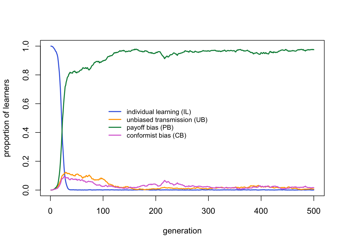
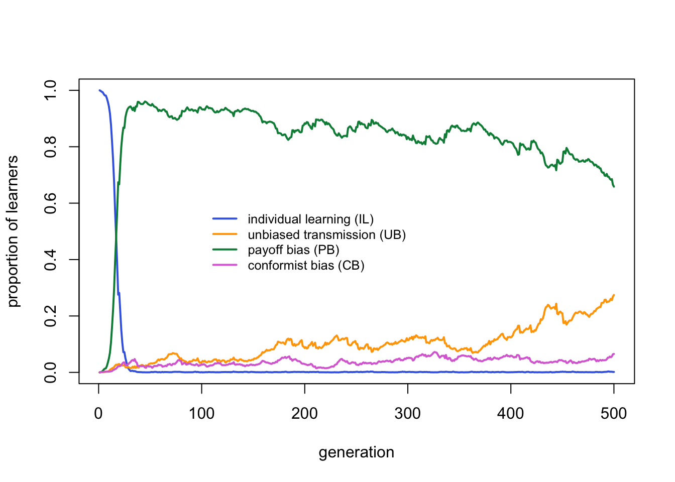
}We can now run the model with default parameter values:
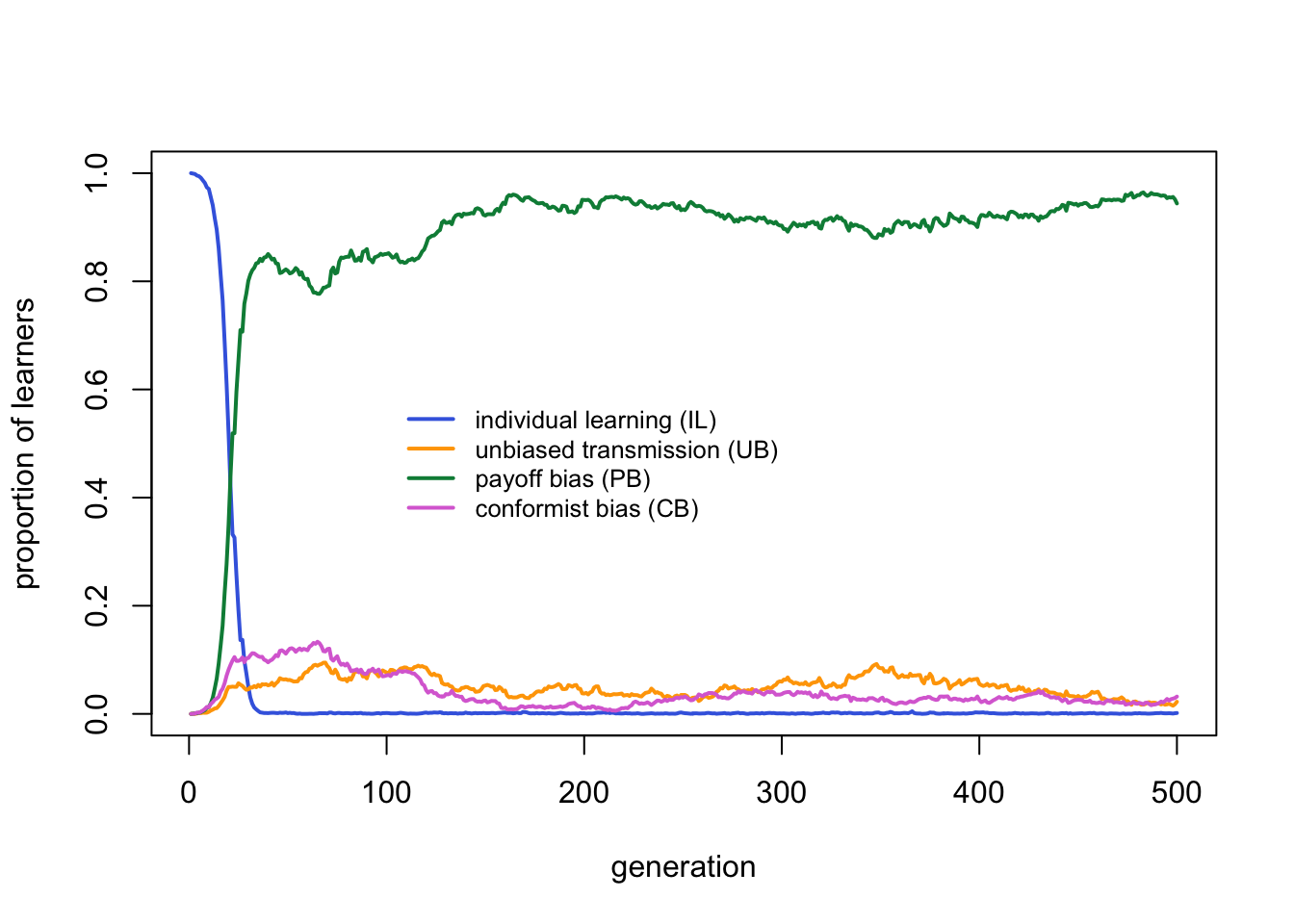
Payoff bias clearly outperforms the other strategies. Individual learning is virtually absent, as expected given that the critical learners all incorporate individual learning. Unbiased and conformist learners each have negligible frequencies.
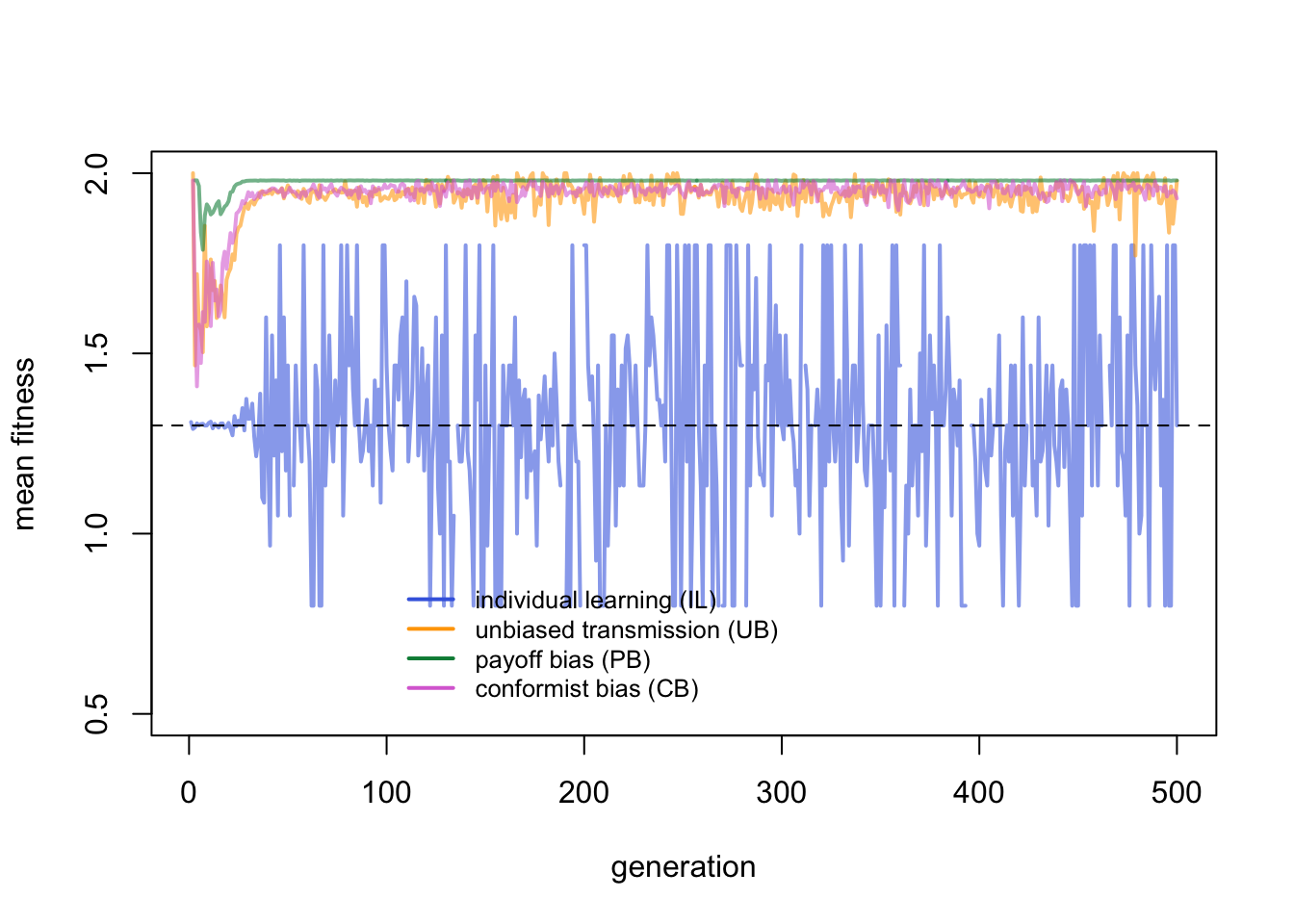
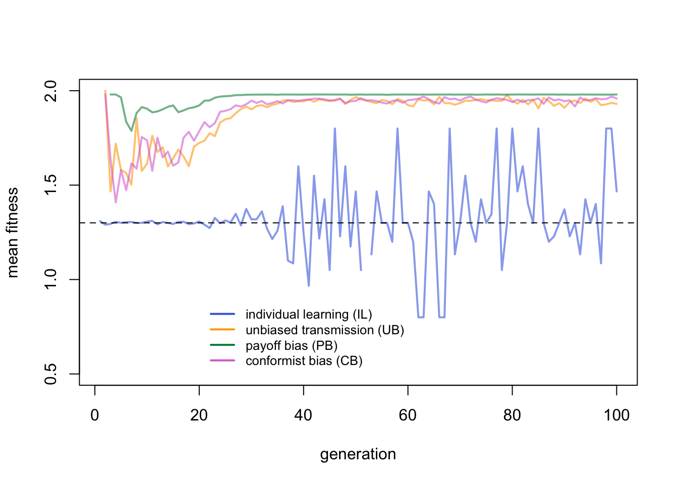
We can plot the fitnesses to explore this further:
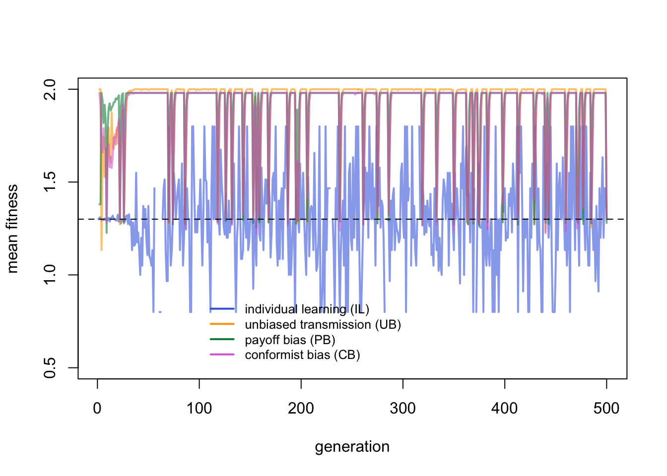
Individual learners fluctuate around their expected mean fitness indicated with the horizontal dotted line. They fluctuate quite wildly given that there are so few of them. The critical learners peak much higher, with drops when the environment changes. Let’s zoom in to the first few generations for a closer look:
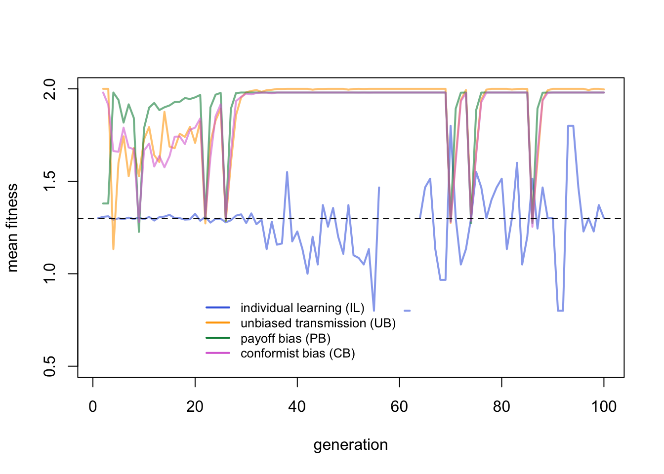
Here the advantage of payoff bias becomes apparent. While UB agents peak slightly higher due to their lower costs of learning, PB agents acquire the correct behaviour quicker after an environmental change than UB and CB agents.
This makes sense. Immediately after an environmental change, all critical learners will be incorrect, and therefore fall back on individual learning. Some will discover the new correct behaviour, others won’t, as determined by \(p_i\). The following generation, critical learners can potentially copy the correct behaviour. PB agents have more chance of copying the correct behaviour amongst their \(n\) demonstrators than UB agents who only copy a single demonstrator, assuming \(n > 1\). CB agents copy the majority of \(n\) demonstrators, but immediately after an environmental change the majority is likely to still be the old, now-incorrect behaviour.
To get an idea of which strategy wins over a range of parameter values and avoid the temptation to cherry-pick particular values, or accidentally miss interesting parts of the parameter space, we can run the simulation over multiple values of two parameters and plot the results in a heat map. The function SLStemporalheatmap takes as its first argument a list of 2 parameters and their values, e.g. list(n = 1:5, v = seq(0.5,1,0.1)), and runs SLStemporal for each parameter value combination. The more values you enter, the higher the resolution of the heatmap (and the longer it takes to run). The winning strategy for each run is the one that exceeds the frequency cutoff after t_max generations. By default cutoff is 0.5. The winning strategy is stored in a matrix called strategy which is then used to create a heatmap with cells coloured according to the winning strategy. If no strategy exceeds cutoff then the cell is coloured grey. To speed things up when running multiple simulations, we reduce \(N\) without much loss of inference.
SLStemporalheatmap <- function(parameters, cutoff = 0.5,
                               N = 1000, t_max = 1000, p_i=0.5, b=1, c_i=0.2, mu=0.001,
                               v=0.9, n=3, f=3, c_c=0.02, c_p=0.02) {

  # for brevity
  p <- parameters

  # list of default arguments
  arguments <- data.frame(N, t_max, p_i, b, c_i, mu, v,
                          n, f, c_c, c_p)

  # for modifying later on
  p1_pos <- which(names(arguments) == names(p[1])) # position of p1 in arguments
  p2_pos <- which(names(arguments) == names(p[2])) # position of p2 in arguments

  # matrix to hold winning strategies
  # 0=none,1=IL,2=UB,3=PB,4=CB
  strategy <- matrix(nrow = length(p[[1]]),
                     ncol = length(p[[2]]))

  for (p1 in p[[1]]) {

    for (p2 in p[[2]]) {

      # set this run's parameter values
      arguments[p1_pos] <- p1
      arguments[p2_pos] <- p2

      # run the model
      output <- SLStemporal(as.numeric(arguments[1]),
                            as.numeric(arguments[2]),
                            as.numeric(arguments[3]),
                            as.numeric(arguments[4]),
                            as.numeric(arguments[5]),
                            as.numeric(arguments[6]),
                            as.numeric(arguments[7]),
                            as.numeric(arguments[8]),
                            as.numeric(arguments[9]),
                            as.numeric(arguments[10]),
                            as.numeric(arguments[11]))

      # record which strategy has frequency above cutoff; if none, set to zero
      if (length(which(output[nrow(output),1:4] > cutoff) > 0)) {
        strategy[which(p[[1]] == p1), which(p[[2]] == p2)] <-
          which(output[nrow(output),1:4] > cutoff)
      } else {
        strategy[which(p[[1]] == p1), which(p[[2]] == p2)] <- 0
      }

    }

  }

  # draw heatmap from strategy
  heatmap(strategy,
          Rowv = NA,
          Colv = NA,
          labRow = p[[1]],
          labCol = p[[2]],
          col = c("grey","royalblue","orange","springgreen4","orchid"),
          breaks = c(-.5,0.5,1.5,2.5,3.5,4.5),
          scale = "none",
          ylab = names(p[1]),
          xlab = names(p[2]))
  legend("bottomleft",
         legend = c("IL", "UB", "PB", "CB"),
         fill = c("royalblue", "orange", "springgreen4","orchid"),
         cex = 0.8,
         bg = "white")

  # export strategy
  strategy

}
Here we create a heatmap across values of \(v\) (rate of environmental change) and \(p_i\) (accuracy of individual learning):
parameters <- list(p_i = seq(0.5,1,0.1), v = seq(0.5,1,0.1))

strategy <- SLStemporalheatmap(parameters)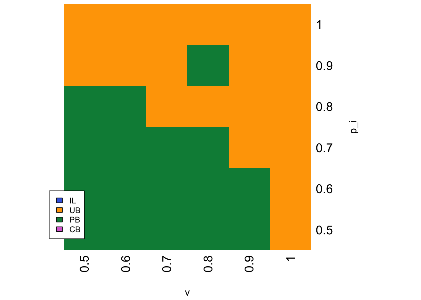
The heatmap above shows that PB is favoured at lower values of \(v\) and \(p_i\), otherwise UB is favoured. This makes sense. When \(v\) is high, environments are relatively stable, and the advantage to PB of more rapidly identifying the new correct behaviour following environmental change is not so useful. UB agents with their lower costs do better once enough critical learners with the correct behaviour have accumulated in the population. Similarly, when \(p_i\) is high, IL agents or critical learners using individual learning can rapidly identify the correct behaviour following an environmental change. UB agents can then copy one of these correct agents at random at a lower cost than PB agents.
Are there any parameter values where CB outperforms PB? This should depend first on the relative cost to CB vs PB:
parameters <- list(c_c = c(0,0.001,0.005,0.01,0.05,0.1),
                   c_p = c(0,0.001,0.005,0.01,0.05,0.1))

strategy <- SLStemporalheatmap(parameters)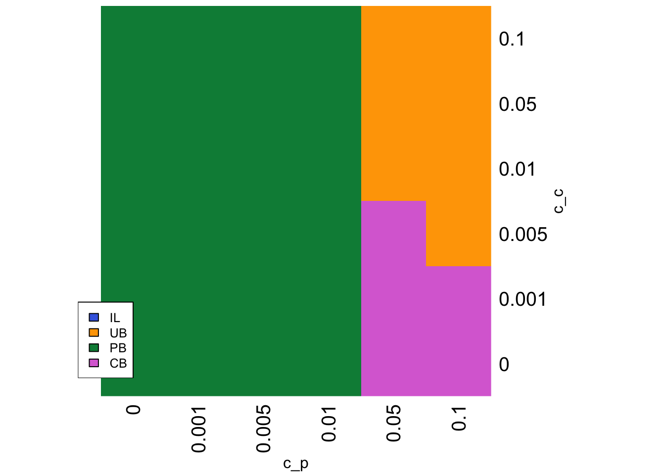
This heatmap shows that CB is favoured when the cost to CB \(c_c\) is low, and the cost to PB \(c_p\) is high (the bottom right of the heatmap). When the cost to both is high then the costless UB is favoured (top right). Otherwise PB is favoured.
If we set the relative cost of PB to be very high such that PB is effectively removed from the simulation, and reduce the cost of CB so that it has a bigger advantage over UB, we can explore the effect of \(n\) and \(f\) on the success of CB:
parameters <- list(n = c(1,3,5,7,9), f = c(1,2,3,5,10))

strategy <- SLStemporalheatmap(parameters, c_p = 0.1, c_c = 0.01)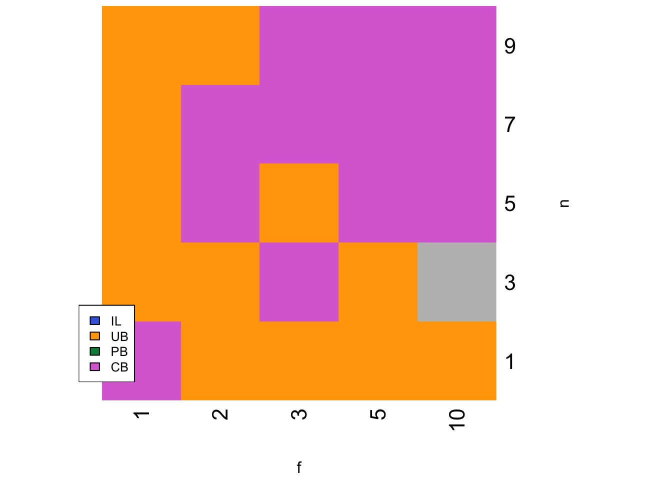
CB is favoured at higher values of \(f\) and \(n\). Given that \(f\) is the strength of conformity, this makes sense. Conformity will also be more effective with more demonstrators (larger \(n\)), as it is more likely that the majority correct behaviour in the entire sub-population is the majority in the sample of \(n\) demonstrators. However, larger \(n\) will also favour payoff bias, which as we have already seen out-performs CB unless \(c_p\) is very large.
Model 19b: Spatially varying environments
Now let’s make environments vary spatially rather than temporally and see if the results change. This situation is similar to Model 7 (migration) where we simulated different groups or sub-populations within the larger population with occasional migration between those groups. We assume here that each group has a different optimal behaviour. The rate of spatial environmental variation is therefore the rate of migration, i.e. the probability that an agent finds themselves in a new group/environment. We remove temporal variation entirely, so optimal behaviours within groups stay the same throughout the simulation.
More specifically, and following Nakahashi et al. (2012), we assume \(G\) groups each containing \(N\) agents, such that there are now \(NG\) agents in total. There are also \(G\) different behaviours labelled 1, 2, 3…\(G\). In each group, one behaviour is correct and all the others are (equally) incorrect. Hence in group 1, behaviour 1 is correct and gives a fitness of \(1 + b\) while behaviours 2 to \(G\) are all incorrect and give a fitness of 1. In group 2, behaviour 2 gives fitness \(1 + b\) and the others give fitness of 1, and so on. There are no behaviours that are incorrect in all groups.
As in Model 7, the rate of migration is \(m\) and migration follows Wright’s island model. Each generation, each agent has a probability \(m\) of being taken out of its group and into a pool of migrants. These migrants are then randomly put back into the now-empty slots ignoring group structure.
Social learning, whether UB, CB or PB, occurs within groups. UB agents pick a single random member of their group to copy, CB agents adopt the majority behaviour amongst \(n\) demonstrators from their group, and PB agents copy the correct behaviour if it is present in at least one of \(n\) demonstrators from their group.
Individual learners are unaffected by spatial environmental variation just as they were unaffected by temporal environmental variation. The critical learners are affected, but differently to temporal variation. Whereas temporal environmental change renders all previous agents’ behaviour incorrect, migrants to a new group can learn from demonstrators who have been in that group previously and potentially already acquired the correct behaviour.
The first step is to create our agent dataframe, this time with a variable group denoting the group id of each agent. Although currently unspecified, the behaviour variable of agent will now hold the numeric behaviour value from 1 to \(G\), rather than 0 or 1. Agents are correct and get a fitness bonus when their behaviour value matches their group id. The output dataframe is identical to Model 19a.
N <- 100
G <- 5
t_max <- 100

# create agents, initially all individual learners
agent <- data.frame(group = rep(1:G, each = N),
                    learning = rep("IL", N*G),
                    behaviour = rep(NA, N*G), # this is now 1,2...G
                    fitness = rep(NA, N*G))

# keep track of freq and fitnesses of each type
output <- data.frame(ILfreq = rep(NA, t_max),
                     UBfreq = rep(NA, t_max),
                     PBfreq = rep(NA, t_max),
                     CBfreq = rep(NA, t_max),
                     ILfitness = rep(NA, t_max),
                     UBfitness = rep(NA, t_max),
                     PBfitness = rep(NA, t_max),
                     CBfitness = rep(NA, t_max))
As before, we first run one generation of individual learning before composing the full set of timestep events. Note the new code for individual learning which is now group-specific. We cycle through each group and set the behaviour to match the group id \(g\) with probability \(p_i\), otherwise another random id from 1 to \(G\) excluding \(g\) (denoted by (1:G)[-g]) with equal probability. Fitness is also group specific, with a bonus only if the agent’s behaviour matches their group. The code for recording type frequency and fitness, and for mutation, are identical to Model 19a except now there are \(NG\) agents rather than \(N\).
t <- 1
p_i <- 0.5
b <- 1
c_i <- 0.2
mu <- 0.5

# individual learning for ILs

# for each group, acquire correct group beh with prob p_i, otherwise random other
for (g in 1:G) {

  ingroup <- agent$learning == "IL" & agent$group == g

  agent$behaviour[ingroup] <- sample(c(g,(1:G)[-g]),
                                     sum(ingroup),
                                     replace = TRUE,
                                     prob = c(p_i, rep((1-p_i)/(G-1), G-1)))

}

# get fitnesses
agent$fitness <- ifelse(agent$behaviour == agent$group, 1 + b, 1)
agent$fitness[agent$learning == "IL"] <- agent$fitness[agent$learning == "IL"] - c_i

head(agent)
## group learning behaviour fitness
## 1 1 IL 1 1.8
## 2 1 IL 1 1.8
## 3 1 IL 1 1.8
## 4 1 IL 1 1.8
## 5 1 IL 5 0.8
## 6 1 IL 5 0.8# record frequencies and fitnesses of each type
output$ILfreq[t] <- sum(agent$learning == "IL") / (N*G)
output$UBfreq[t] <- sum(agent$learning == "UB") / (N*G)
output$PBfreq[t] <- sum(agent$learning == "PB") / (N*G)
output$CBfreq[t] <- sum(agent$learning == "CB") / (N*G)
output$ILfitness[t] <- mean(agent$fitness[agent$learning == "IL"])
output$UBfitness[t] <- mean(agent$fitness[agent$learning == "UB"])
output$PBfitness[t] <- mean(agent$fitness[agent$learning == "PB"])
output$CBfitness[t] <- mean(agent$fitness[agent$learning == "CB"])
head(output)## ILfreq UBfreq PBfreq CBfreq ILfitness UBfitness PBfitness CBfitness
## 1 1 0 0 0 1.336 NaN NaN NaN
## 2 NA NA NA NA NA NA NA NA
## 3 NA NA NA NA NA NA NA NA
## 4 NA NA NA NA NA NA NA NA
## 5 NA NA NA NA NA NA NA NA
## 6 NA NA NA NA NA NA NA NA# mutation
mutate <- runif(N) < mu
IL_mutate <- agent$learning == "IL" & mutate
UB_mutate <- agent$learning == "UB" & mutate
PB_mutate <- agent$learning == "PB" & mutate
CB_mutate <- agent$learning == "CB" & mutate
agent$learning[IL_mutate] <- sample(c("UB","PB","CB"), sum(IL_mutate), replace = TRUE)
agent$learning[UB_mutate] <- sample(c("IL","PB","CB"), sum(UB_mutate), replace = TRUE)
agent$learning[PB_mutate] <- sample(c("IL","UB","CB"), sum(PB_mutate), replace = TRUE)
agent$learning[CB_mutate] <- sample(c("IL","UB","PB"), sum(CB_mutate), replace = TRUE)Now we can start the sequence of within-generation events. First we record the previous agent dataframe and do individual learning, as above.
t <- 2

# 1. store previous timestep agent
previous_agent <- agent

# 2. individual learning for ILs

# for each group, acquire correct group beh with prob p_i, otherwise random other
for (g in 1:G) {

  ingroup <- agent$learning == "IL" & agent$group == g

  agent$behaviour[ingroup] <- sample(c(g,(1:G)[-g]),
                                     sum(ingroup),
                                     replace = TRUE,
                                     prob = c(p_i, rep((1-p_i)/(G-1), G-1)))

}
Next is social learning. Now that demonstrators must come from the agent’s own group, we need slightly more complex code to create the dems dataframe. The following code cycles through each group, samples \(n\) demonstrators for each agent within that group, and adds them to the dems matrix using the rbind command.
n <- 3

# 3. social learning for critical learners

# select group-specific demonstrators
dems <- NULL

# cycle through each group
for (g in 1:G) {

  ingroup <- agent$group == g

  dems <- rbind(dems,
                matrix(data = sample(previous_agent$behaviour[ingroup], N*n, replace = TRUE),
                       nrow = N, ncol = n))

}

head(dems)
## [,1] [,2] [,3]
## [1,] 1 5 1
## [2,] 4 1 1
## [3,] 5 3 1
## [4,] 1 2 5
## [5,] 1 3 1
## [6,] 1 1 1UB agents copy the first demonstrator stored in the first column of dems. As before, there is no directional change in the frequency of correct behaviour due to UB.
# proportion correct before social learning
mean(agent$behaviour[agent$learning == "UB"] == agent$group[agent$learning == "UB"])
## [1] 0.5316456# for UBs, copy the behaviour of the 1st dem in dems
agent$behaviour[agent$learning == "UB"] <- dems[agent$learning == "UB", 1]
# proportion correct after social learning
mean(agent$behaviour[agent$learning == "UB"] == agent$group[agent$learning == "UB"])## [1] 0.4810127PB agents copy the correct behaviour in their group if at least one demonstrator has the correct behaviour, otherwise they copy their first (incorrect) random demonstrator. Here PB_correct identifies PB agents who observe at least one correct demonstrator, and PB_incorrect identifies PB agents who observe all incorrect demonstrators.
# proportion correct before social learning
mean(agent$behaviour[agent$learning == "PB"] == agent$group[agent$learning == "PB"])
## [1] 0.5113636# for PB, copy correct if at least one of dems is correct
PB_correct <- agent$learning == "PB" & rowSums(dems == agent$group) > 0
PB_incorrect <- agent$learning == "PB" & rowSums(dems == agent$group) == 0
agent$behaviour[PB_correct] <- agent$group[PB_correct]
agent$behaviour[PB_incorrect] <- dems[PB_incorrect, 1]
# proportion correct after social learning
mean(agent$behaviour[agent$learning == "PB"] == agent$group[agent$learning == "PB"])## [1] 0.8636364As in Model 19a, you should see the frequency of correct behaviours increase after payoff biased copying.
Finally CB agents are disproportionately more likely to copy the majority trait amongst the demonstrators. Because there are now potentially more than two behaviours when \(G > 2\), we need to calculate the number of times each trait appears amongst the \(n\) demonstrators for each agent (stored in counts), get copy probabilities for each trait based on the counts and Equation 17.2 (stored in copy_probs), then actually pick a trait based on these probabilities using apply on copy_probs.
f <- 3

# proportion correct before social learning
mean(agent$behaviour[agent$learning == "CB"] == agent$group[agent$learning == "CB"])
## [1] 0.6025641# for CB, copy majority behaviour according to parameter f
# get number of times each trait appears in n dems for each agent
counts <- matrix(nrow = N*G, ncol = G)
for (g in 1:G) counts[,g] <- rowSums(dems == g)
# get copy probs based on counts and f
copy_probs <- matrix(nrow = N*G, ncol = G)
for (g in 1:G) copy_probs[,g] <- rowSums(dems == g)^f / rowSums(counts^f)
# pick a trait based on copy_probs
CB_beh <- apply(copy_probs, 1, function(x) sample(1:G, 1, prob = x))
# CB agents copy the trait
agent$behaviour[agent$learning == "CB"] <- CB_beh[agent$learning == "CB"]
# proportion correct after social learning
mean(agent$behaviour[agent$learning == "CB"] == agent$group[agent$learning == "CB"])## [1] 0.6794872As in Model 19a, CB is unlikely to have increased the frequency of correct behaviours by much, if at all.
Steps 4, 5 and 6 are similar to before: incorrect critical learners engage in individual learning, fitnesses are calculated, and frequencies and mean fitness of each type are recorded in output.
c_c <- 0.02
c_p <- 0.02

# 4. incorrect social learners engage in individual learning
incorrect_SL <- agent$learning != "IL" & agent$behaviour != agent$group

for (g in 1:G) {

  ingroup <- incorrect_SL & agent$group == g

  agent$behaviour[ingroup] <- sample(c(g,(1:G)[-g]),
                                     sum(ingroup),
                                     replace = TRUE,
                                     prob = c(p_i, rep((1-p_i)/(G-1), G-1)))

}

# 5. calculate fitnesses

# all correct agents get bonus b
agent$fitness <- ifelse(agent$behaviour == agent$group, 1 + b, 1)

# costs of learning
agent$fitness[agent$learning == "IL"] <- agent$fitness[agent$learning == "IL"] - c_i
agent$fitness[agent$learning == "PB"] <- agent$fitness[agent$learning == "PB"] - c_p
agent$fitness[agent$learning == "CB"] <- agent$fitness[agent$learning == "CB"] - c_c
agent$fitness[incorrect_SL] <- agent$fitness[incorrect_SL] - c_i

# 6. record frequencies and fitnesses of each type
output$ILfreq[t] <- sum(agent$learning == "IL") / (N*G)
output$UBfreq[t] <- sum(agent$learning == "UB") / (N*G)
output$PBfreq[t] <- sum(agent$learning == "PB") / (N*G)
output$CBfreq[t] <- sum(agent$learning == "CB") / (N*G)
output$ILfitness[t] <- mean(agent$fitness[agent$learning == "IL"])
output$UBfitness[t] <- mean(agent$fitness[agent$learning == "UB"])
output$PBfitness[t] <- mean(agent$fitness[agent$learning == "PB"])
output$CBfitness[t] <- mean(agent$fitness[agent$learning == "CB"])

head(output)
## ILfreq UBfreq PBfreq CBfreq ILfitness UBfitness PBfitness CBfitness
## 1 1.00 0.000 0.000 0.000 1.336000 NaN NaN NaN
## 2 0.51 0.158 0.176 0.156 1.290196 1.617722 1.884545 1.762051
## 3 NA NA NA NA NA NA NA NA
## 4 NA NA NA NA NA NA NA NA
## 5 NA NA NA NA NA NA NA NA
## 6 NA NA NA NA NA NA NA NAStep 7 is selection and reproduction. We make this occur within groups; if social learning occurs within groups, it makes sense that mating and reproduction also happens within groups.
##
##    CB    IL    PB    UB
## 0.156 0.510 0.176 0.158
# 7. selection and reproduction
# (now within-group)
for (g in 1:G) {
ingroup <- agent$group == g
relative_fitness <- agent$fitness[ingroup] / sum(agent$fitness[ingroup])
agent$learning[ingroup] <- sample(agent$learning[ingroup],
N,
prob = relative_fitness,
replace = TRUE)
}
# after selection
table(agent$learning)/(N*G)##
## CB IL PB UB
## 0.170 0.418 0.238 0.174Next is mutation, identical to above, and finally some new code implementing migration. Just as in Model 4, we select migrants with probability \(m\) per agent, add these migrants’ learning type and behaviour to a migrants dataframe, then put these randomly back into the migrant slots ignoring group id.
m <- 0.1

# 8. mutation
mutate <- runif(N*G) < mu
IL_mutate <- agent$learning == "IL" & mutate
UB_mutate <- agent$learning == "UB" & mutate
PB_mutate <- agent$learning == "PB" & mutate
CB_mutate <- agent$learning == "CB" & mutate

agent$learning[IL_mutate] <- sample(c("UB","PB","CB"), sum(IL_mutate), replace = TRUE)
agent$learning[UB_mutate] <- sample(c("IL","PB","CB"), sum(UB_mutate), replace = TRUE)
agent$learning[PB_mutate] <- sample(c("IL","UB","CB"), sum(PB_mutate), replace = TRUE)
agent$learning[CB_mutate] <- sample(c("IL","UB","PB"), sum(CB_mutate), replace = TRUE)

# 9. migration

# NG probabilities, one for each agent, to compare against m
probs <- runif(1:(N*G))

# with prob m, add an agent's learning and behaviour to list of migrants
migrants <- agent[probs < m, c("learning", "behaviour")]

# put migrants randomly into empty slots
agent[probs < m, c("learning", "behaviour")] <- migrants[sample(rownames(migrants)),]
The following function SLSspatial combines all these code chunks:
SLSspatial <- function(N=1000, t_max=500, p_i=0.5, b=1, c_i=0.2, mu=0.001,
                       G=5, n=3, f=3, c_c=0.02, c_p=0.02, m=0.1) {

  # create agents, initially all individual learners
  agent <- data.frame(group = rep(1:G, each = N),
                      learning = rep("IL", N*G),
                      behaviour = rep(NA, N*G), # this is now 1,2...G
                      fitness = rep(NA, N*G))

  # keep track of freq and fitnesses of each type
  output <- data.frame(ILfreq = rep(NA, t_max),
                       UBfreq = rep(NA, t_max),
                       PBfreq = rep(NA, t_max),
                       CBfreq = rep(NA, t_max),
                       ILfitness = rep(NA, t_max),
                       UBfitness = rep(NA, t_max),
                       PBfitness = rep(NA, t_max),
                       CBfitness = rep(NA, t_max))

  # start timestep loop
  for (t in 1:t_max) {

    # 1. store previous timestep agent
    previous_agent <- agent

    # 2. individual learning for ILs

    # for each group, acquire correct group beh with prob p_i, otherwise random other
    for (g in 1:G) {

      ingroup <- agent$learning == "IL" & agent$group == g

      agent$behaviour[ingroup] <- sample(c(g,(1:G)[-g]),
                                         sum(ingroup),
                                         replace = TRUE,
                                         prob = c(p_i, rep((1-p_i)/(G-1), G-1)))

    }

    # 3. social learning for social learners

    # skip if no social learners
    if (sum(agent$learning == "IL") < N*G) {

      # select group-specific demonstrators
      dems <- NULL

      # cycle through each group
      for (g in 1:G) {

        ingroup <- agent$group == g

        dems <- rbind(dems,
                      matrix(data = sample(previous_agent$behaviour[ingroup], N*n, replace = TRUE),
                             nrow = N, ncol = n))

      }

      # for UBs, copy the behaviour of the 1st dem in dems
      agent$behaviour[agent$learning == "UB"] <- dems[agent$learning == "UB", 1]

      # for PB, copy correct group beh if at least one of dems is correct
      PB_correct <- agent$learning == "PB" & rowSums(dems == agent$group) > 0
      PB_incorrect <- agent$learning == "PB" & rowSums(dems == agent$group) == 0

      agent$behaviour[PB_correct] <- agent$group[PB_correct]
      agent$behaviour[PB_incorrect] <- dems[PB_incorrect, 1]

      # for CB, copy majority behaviour according to parameter f

      # get number of times each trait appears in n dems for each agent
      counts <- matrix(nrow = N*G, ncol = G)
      for (g in 1:G) counts[,g] <- rowSums(dems == g)

      # get copy probs based on counts and f
      copy_probs <- matrix(nrow = N*G, ncol = G)
      for (g in 1:G) copy_probs[,g] <- rowSums(dems == g)^f / rowSums(counts^f)

      # pick a trait based on copy_probs
      CB_beh <- apply(copy_probs, 1, function(x) sample(1:G, 1, prob = x))

      # CB agents copy the trait
      agent$behaviour[agent$learning == "CB"] <- CB_beh[agent$learning == "CB"]

    }

    # 4. incorrect social learners engage in individual learning
    incorrect_SL <- agent$learning != "IL" & agent$behaviour != agent$group

    for (g in 1:G) {

      ingroup <- incorrect_SL & agent$group == g

      agent$behaviour[ingroup] <- sample(c(g,(1:G)[-g]),
                                         sum(ingroup),
                                         replace = TRUE,
                                         prob = c(p_i, rep((1-p_i)/(G-1), G-1)))

    }

    # 5. calculate fitnesses

    # all correct agents get bonus b
    agent$fitness <- ifelse(agent$behaviour == agent$group, 1 + b, 1)

    # costs of learning
    agent$fitness[agent$learning == "IL"] <- agent$fitness[agent$learning == "IL"] - c_i
    agent$fitness[agent$learning == "PB"] <- agent$fitness[agent$learning == "PB"] - c_p
    agent$fitness[agent$learning == "CB"] <- agent$fitness[agent$learning == "CB"] - c_c
    agent$fitness[incorrect_SL] <- agent$fitness[incorrect_SL] - c_i

    # 6. record frequencies and fitnesses of each type
    output$ILfreq[t] <- sum(agent$learning == "IL") / (N*G)
    output$UBfreq[t] <- sum(agent$learning == "UB") / (N*G)
    output$PBfreq[t] <- sum(agent$learning == "PB") / (N*G)
    output$CBfreq[t] <- sum(agent$learning == "CB") / (N*G)
    output$ILfitness[t] <- mean(agent$fitness[agent$learning == "IL"])
    output$UBfitness[t] <- mean(agent$fitness[agent$learning == "UB"])
    output$PBfitness[t] <- mean(agent$fitness[agent$learning == "PB"])
    output$CBfitness[t] <- mean(agent$fitness[agent$learning == "CB"])

    # 7. selection and reproduction
    # (now within-group)

    for (g in 1:G) {

      ingroup <- agent$group == g

      relative_fitness <- agent$fitness[ingroup] / sum(agent$fitness[ingroup])

      agent$learning[ingroup] <- sample(agent$learning[ingroup],
                                        N,
                                        prob = relative_fitness,
                                        replace = TRUE)

    }

    # 8. mutation
    mutate <- runif(N*G) < mu
    IL_mutate <- agent$learning == "IL" & mutate
    UB_mutate <- agent$learning == "UB" & mutate
    PB_mutate <- agent$learning == "PB" & mutate
    CB_mutate <- agent$learning == "CB" & mutate

    agent$learning[IL_mutate] <- sample(c("UB","PB","CB"), sum(IL_mutate), replace = TRUE)
    agent$learning[UB_mutate] <- sample(c("IL","PB","CB"), sum(UB_mutate), replace = TRUE)
    agent$learning[PB_mutate] <- sample(c("IL","UB","CB"), sum(PB_mutate), replace = TRUE)
    agent$learning[CB_mutate] <- sample(c("IL","UB","PB"), sum(CB_mutate), replace = TRUE)

    # 9. migration

    # NG probabilities, one for each agent, to compare against m
    probs <- runif(1:(N*G))

    # with prob m, add an agent's learning and behaviour to list of migrants
    migrants <- agent[probs < m, c("learning", "behaviour")]

    # put migrants randomly into empty slots
    agent[probs < m, c("learning", "behaviour")] <- migrants[sample(rownames(migrants)),]

  }

  # add predicted IL fitness to output and export
  output$predictedILfitness <- 1 + b*p_i - c_i
  output

}
The plotting functions SLSfreqplot and SLSfitnessplot work fine for SLSspatial. Here is a default run:
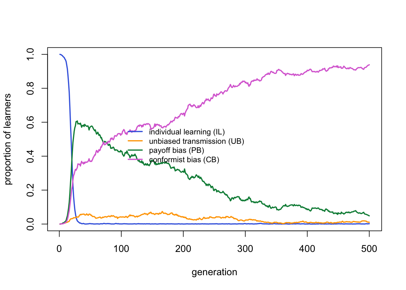
As before, PB is favoured over all other strategies. The fitness plot, however, looks different:
And zooming in on the first few generations:
Whereas in the temporal model we could see PB agents adjusting more rapidly to periodic environmental change events, here PB agents gain an advantage at the start and keep that advantage throughout. This is because migration occurs at a constant rate. Every generation a fraction \(m\) of agents move to a random group. These migrants will be incorrect in their new environment. PB agents have a better chance that one of their \(n\) demonstrators will be correct than UB agents who only copy a single demonstrator, who might be an incorrect migrant.
CB agents, perhaps surprisingly, do no better than UB agents. As long as \(m\) is not too high, the majority of agents in each group will remain correct, and CB migrants can adopt this correct majority behaviour. But even with \(f > 1\), conformity is still probabilistic, and with only \(n = 3\) demonstrators there is a chance that the majority amongst \(N\) agents is not the majority amongst \(n\).
So let’s increase \(f\) to increase our chances of picking the majority trait, and increase \(n\) to increase the chances that the correct behaviour is the majority. We also make the cost to CB slightly less than that to PB.
Now CB is favoured over PB. Whereas in temporally varying environments CB was only favoured when the costs to PB were so high as to remove PB from the competition, here CB is favoured when its costs are only slightly lower than PB. We can confirm this by running the temporal model with the same parameter values:
For the same parameter values, CB agents do much better relative to PB agents in spatially varying environments than in temporally varying environments.
As in Model 19a, heatmaps across several parameter values can give a broader understanding of the model dynamics. The heatmap function needs to be modified given that SLSspatial has different parameters to SLStemporal, like so:
SLSspatialheatmap <- function(parameters, cutoff = 0.5,
                              N = 500, t_max = 1000, p_i=0.5, b=1, c_i=0.2, mu=0.001,
                              G=5, n=3, f=3, c_c=0.02, c_p=0.02, m=0.1) {

  # for brevity
  p <- parameters

  # list of default arguments
  arguments <- data.frame(N, t_max, p_i, b, c_i, mu,
                          G, n, f, c_c, c_p, m)

  # for modifying later on
  p1_pos <- which(names(arguments) == names(p[1])) # position of p1 in arguments
  p2_pos <- which(names(arguments) == names(p[2])) # position of p2 in arguments

  # matrix to hold winning strategies
  # 0=none,1=IL,2=UB,3=PB,4=CB
  strategy <- matrix(nrow = length(p[[1]]),
                     ncol = length(p[[2]]))

  for (p1 in p[[1]]) {

    for (p2 in p[[2]]) {

      # set this run's parameter values
      arguments[p1_pos] <- p1
      arguments[p2_pos] <- p2

      # run the model
      output <- SLSspatial(as.numeric(arguments[1]),
                           as.numeric(arguments[2]),
                           as.numeric(arguments[3]),
                           as.numeric(arguments[4]),
                           as.numeric(arguments[5]),
                           as.numeric(arguments[6]),
                           as.numeric(arguments[7]),
                           as.numeric(arguments[8]),
                           as.numeric(arguments[9]),
                           as.numeric(arguments[10]),
                           as.numeric(arguments[11]),
                           as.numeric(arguments[12]))

      # record which strategy has frequency above cutoff; if none, set to zero
      if (length(which(output[nrow(output),1:4] > cutoff) > 0)) {
        strategy[which(p[[1]] == p1), which(p[[2]] == p2)] <-
          which(output[nrow(output),1:4] > cutoff)
      } else {
        strategy[which(p[[1]] == p1), which(p[[2]] == p2)] <- 0
      }

    }

  }

  # draw heatmap from strategy
  heatmap(strategy,
          Rowv = NA,
          Colv = NA,
          labRow = p[[1]],
          labCol = p[[2]],
          col = c("grey","royalblue","orange","springgreen4","orchid"),
          breaks = c(-.5,0.5,1.5,2.5,3.5,4.5),
          scale = "none",
          ylab = names(p[1]),
          xlab = names(p[2]))
  legend("bottomleft",
         legend = c("IL", "UB", "PB", "CB"),
         fill = c("royalblue", "orange", "springgreen4","orchid"),
         cex = 0.8,
         bg = "white")

  # export strategy
  strategy

}
Whereas in Model 19a we varied \(v\), the rate of environmental change, we now vary \(m\), the equivalent parameter controlling the rate of spatial environmental change experienced by each agent (i.e. their probability of migrating to a new environment), along with the accuracy of individual learning \(p_i\):
parameters <- list(p_i = seq(0.5,1,0.1),
                   m = c(0,0.05,0.1,0.15,0.2))

strategy <- SLSspatialheatmap(parameters)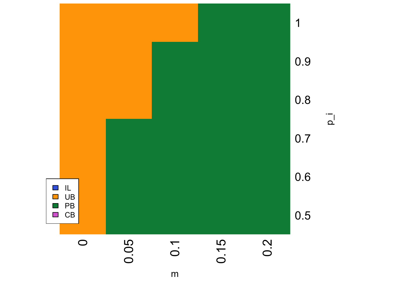
PB is favoured when \(m\) is relatively large and \(p_i\) is relatively low. When \(m = 0\) there is no migration and hence no environmental change. Just as for stable environments in Model 19a, UB agents are favoured because the correct behaviour quickly spreads in each sub-population and UB agents can copy this correct behaviour at lower cost than the other strategies. As migration increases, PB agents do better than UB agents when they migrate because of their larger pool of demonstrators when \(n > 1\). Similarly, as \(p_i\) increases then the correct behaviour becomes more common even amongst migrants, such that UB agents can easily copy the correct behaviour at lower cost than PB and CB.
Above we determined that CB agents do well when \(f\) and \(n\) are both large, and the cost of CB is slightly lower than those of PB. Here we can test this more thoroughly:
parameters <- list(n = c(3,5,7,9), f = c(1,3,5,7))

strategy <- SLSspatialheatmap(parameters, c_c = 0.01)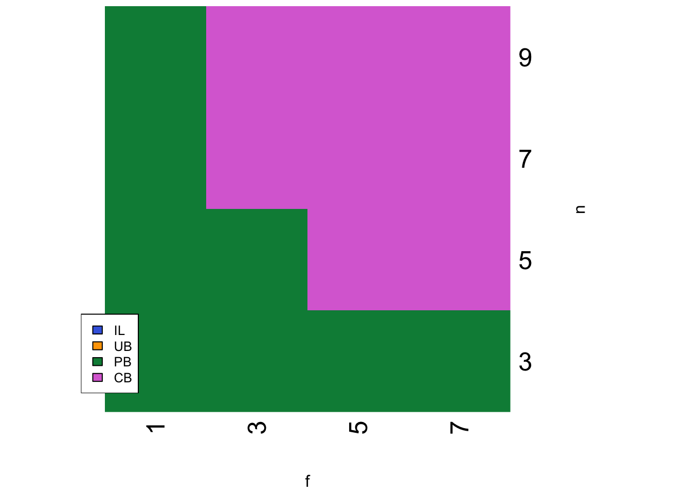
When CB is only slightly less costly than PB, and \(f\) and \(n\) are sufficiently large, then CB is favoured. For the same parameter values in the temporal model, CB is never favoured.
Summary
Model 19 examined the evolution of two commonly studied social learning strategies, payoff bias (PB) and conformist bias (CB), relative to unbiased transmission (UB) and individual learning (IL). Model 19a found that in temporally varying environments PB is widely favoured, unless environments are very stable or individual learning is very accurate in which case UB is favoured. UB is favoured in these cases because correct behaviour becomes very common, allowing UB agents to copy the correct behaviour at lower cost than PB. When correct behaviour is less common then PB agents have the advantage of being able to identify that correct behaviour more effectively by learning from multiple demonstrators. CB is only favoured in temporally varying environments when the costs to PB are so high as to effectively remove them from the population. This recreates the findings of a similar mathematical model by Nakahashi et al. (2012) who concluded that “[CB is] not very important in a temporally varying environment, especially when [PB] are in the mix” (p.406).
In spatially varying environments, PB is also widely favoured unless environments are stable (i.e. there is no migration) or individual learning is very accurate, in which case UB again is favoured. However, CB is much more widely favoured in spatially varying environments than temporally varying environments. CB is favoured when its costs are only slightly less than those of PB, and when the strength of conformity (\(f\)) and number of demonstrators (\(n\)) are reasonably large. Under these conditions migrating CB agents can take advantage of the majority correct behaviour that is found in each group. This again recreates the analytical findings of Nakahashi et al. (2012) who state that “If the cost to [PB] is larger than that to [CB], [PB] never evolve” (p.406).
The recreation of findings from Nakahashi et al. (2012) is reassuring given that Model 19 is an agent-based simulation and theirs is an analytical model. There are also several other differences: they modelled pure social learning strategies whereas we modelled critical learners who combine social and individual learning; their conformity and payoff bias involved learning from every member of the population rather than a sample (i.e. in their model \(n = N\)), and they set the strength of conformity to infinity so agents always picked the majority. Nevertheless, the major findings are the same. If the same findings come from different modelling approaches and assumptions, we can be more confident in their reliability. Other similar models include Henrich & Boyd (1998) and Kendal et al. (2009); for a review see Aoki & Feldman (2014).
The finding that conformity should be used when environments vary spatially rather than temporally has been supported experimentally by Deffner et al. (2020), who found that participants used conformist social learning more often after migrating to a new group than when environments changed globally. Deffner et al. (2020) used the same formulation of conformity as used here and provide a mean estimate from their participants of \(f = 3.30\), suggesting reasonably strong but not excessively strong conformity. They also found that participants often targeted fellow participants who had been in their groups for the longest. This was not possible in our model given that the \(n\) demonstrators were picked at random. However, non-random demonstrator selection (effectively, the indirectly biased transmission of Model 4) would be an interesting extension. Conformity following migration is a form of acculturation, which has major consequences for the maintenance of between-group cultural variation (see Henrich & Boyd 1998; Mesoudi 2018).
The success of CB in spatially varying environments hinges on whether it is less costly than PB. Is this a plausible assumption? Nakahashi et al. (2012) think so, arguing that “[t]his assumption seems plausible, given that [PB] have a more complicated task than [CB], which involves assessing payoffs or at least relative payoff differences for the cultural traits present.” (p.405). While that may be the case, tallying the frequencies of multiple traits across multiple demonstrators also seems quite costly. Empirically quantifying the costs of social learning strategies such as CB and PB would be a worthwhile endeavour.
In terms of programming, much of the code here is recycled from previous models that have examined unbiased, conformist and payoff/directly biased cultural transmission, as well as Model 18 which simulated the basic UB critical learners. The major addition is the use of a heatmap to explore a wide parameter space. This can be more effective than cherry-picking particular parameter values, and provide a good visualisation of how two parameters interact. The limitation is that you still have to pick upper and lower parameter bounds, and you can only examine two parameters at a time (3D parameter space plots are possible but hard to interpret).
Exercises
Rather than fixed costs to CB and PB, it seems more plausible to assume that the costs of conformity and payoff bias increase with \(n\). Calculating the majority or identifying the correct behaviour amongst 100 demonstrators would take more time and effort than calculating the majority or identifying the correct behaviour amongst 3 demonstrators. To be comparable with UB agents, who pay no cost for locating a single random agent as a demonstrator, rewrite Model 19 to give CB and PB agents the first demonstrator for free, then penalise the remaining \(n - 1\) demonstrators at \(c_c\) and \(c_p\) per demonstrator, i.e. \(- c_c(n-1)\) and \(- c_p(n-1)\) respectively. These increasing costs should introduce an interesting trade-off, given that CB and PB both work better with more demonstrators, but will also incur greater costs of learning.
Nakahashi et al. (2012) found that conformity is more likely to evolve in spatially varying environments as the number of traits increases. In Model 19b a single parameter \(G\) controls both the number of groups and the number of traits/behaviours. First, vary \(G\) under conditions that generally favour conformity to see whether Nakahashi et al.’s conclusion also holds here. Second, separate the number of groups and the number of traits into two independent parameters. Does increasing the number of traits increase the likelihood of conformity evolving independently of the number of groups?
In Model 19 \(f\) and \(n\) are fixed at the same value throughout the simulation. Modify Model 19 to make them evolve alongside the learning strategies. Each agent should have a different \(f\) and \(n\) initially drawn from a uniform or normal distribution. Then just as agents currently reproduce their learning strategy based on their relative fitness, make them also reproduce their value of \(f\) (for CB agents) and \(n\) (for PB and CB agents). Add mutation to \(f\) and \(n\) as well. In line with our observations that the strength of CB and PB increase with increasing \(n\) and \(f\), do these parameters evolve upwards throughout the simulation? (NB you might want to set an upper limit to avoid excessive run times) What if you make the cost of PB and CB depend on \(n\), as per Exercise 1 above?
References
Aoki, K., & Feldman, M. W. (2014). Evolution of learning strategies in temporally and spatially variable environments: a review of theory. Theoretical Population Biology, 91, 3-19.
Deffner, D., Kleinow, V., & McElreath, R. (2020). Dynamic social learning in temporally and spatially variable environments. Royal Society Open Science, 7(12), 200734.
Enquist, M., Eriksson, K., & Ghirlanda, S. (2007). Critical social learning: a solution to Rogers’s paradox of nonadaptive culture. American Anthropologist, 109(4), 727-734.
Henrich, J., & Boyd, R. (1998). The evolution of conformist transmission and the emergence of between-group differences. Evolution and Human Behavior, 19(4), 215-241.
Kendal, J., Giraldeau, L. A., & Laland, K. (2009). The evolution of social learning rules: payoff-biased and frequency-dependent biased transmission. Journal of Theoretical Biology, 260(2), 210-219.
Laland, K. N. (2004). Social learning strategies. Animal Learning & Behavior, 32(1), 4-14.
Mesoudi, A. (2018). Migration, acculturation, and the maintenance of between-group cultural variation. PloS one, 13(10), e0205573.
Nakahashi, W., Wakano, J. Y., & Henrich, J. (2012). Adaptive social learning strategies in temporally and spatially varying environments: How temporal vs. spatial variation, number of cultural traits, and costs of learning influence the evolution of conformist-biased transmission, payoff-biased transmission, and individual learning. Human Nature, 23, 386-418.