Model 13: Social contagion
Introduction
Model 13, Model 14 and Model 15 concern the linked topics of social contagion, social networks and opinion formation. These models and topics do not originate in the field of cultural evolution. They come instead from sociology and epidemiology. However, we will see how some of these concepts and models have direct parallels in the cultural evolution concepts and models we have already covered in this series. We will also see how they extend cultural evolution models in useful ways.
Social contagion models draw a parallel between the spread of diseases from person to person and the spread of ideas, beliefs, products, technologies and other cultural traits from person to person. Just as you can catch a disease like influenza or covid from another person, so too can you be ‘infected’ with their ideas, beliefs or habits through exposure to them in the form of observation or conversation.
While this analogy between diseases and ideas has merit, we should be wary of its limitations. For example, diseases can be caught with a single exposure to an infected individual, whereas many ideas, skills or beliefs require repeated exposure, such as when persuasion is needed to convince someone of an unusual belief or idea, or when a skill requires a lengthy apprenticeship to master. Nevertheless, contagion models from epidemiology provide useful insights into how cultural traits spread through society.
Model 13a: The SI model
Contagion models originating in epidemiology are called ‘compartmental’ models (Anderson & May 1992). They place individuals in one of a set of compartments. The simplest model compartmentalises individuals as either Susceptible (S) to acquiring a disease (or cultural trait), or already Infected (I) with the disease (or cultural trait). Consequently, these are called SI models.
Model 13a simulates the simplest possible SI model. We assume \(N\) agents, each of whom can be Susceptible or Infected. In each generation from 1 to \(t_{max}\), every agent interacts with a single randomly chosen other agent in the population. If that other agent (the ‘demonstrator’) is Infected, then the focal agent becomes Infected with probability \(\beta\). This parameter \(\beta\) represents the ‘transmissability’ of the cultural trait, with direct analogy to the transmissability of a disease. If the focal agent is already Infected, then nothing changes. The population is fixed, i.e. agents do not recover, die or migrate, and unstructured, i.e. any agent can potentially infect any other agent in the population in any timestep.
The function below implements this SI model. We specify an initial frequency of agents who are Infected with the parameter \(I_0\), as in the absence of mutation the trait would otherwise never appear. We have \(r_{max}\) independent runs, and plot the proportion of Infected agents over time.
SImodel <- function(N, beta, I_0, t_max, r_max) {

  # create a matrix with t_max rows and r_max columns, fill with NAs, convert to dataframe
  output <- as.data.frame(matrix(NA, t_max, r_max))

  # purely cosmetic: rename the columns with run1, run2 etc.
  names(output) <- paste("run", 1:r_max, sep="")

  for (r in 1:r_max) {

    # create first generation
    agent <- data.frame(trait = sample(c("I","S"), N, replace = TRUE,
                                     prob = c(I_0,1-I_0)))

    # add first generation's frequency of I to first row of column run
    output[1,r] <- sum(agent$trait == "I") / N

    for (t in 2:t_max) {

      # copy agent to previous_agent dataframe
      previous_agent <- agent

      # for each agent, pick a random agent from the previous generation
      # as demonstrator and store their trait
      demonstrator_trait <- sample(previous_agent$trait, N, replace = TRUE)

      # get N random numbers each between 0 and 1
      copy <- runif(N)

      # if agent is S, demonstrator is I and with probability beta, acquire I
      agent$trait[previous_agent$trait == "S" &
                  demonstrator_trait == "I" &
                  copy < beta] <- "I"

      # get frequency of I and put it into output slot for this generation t and run r
      output[t,r] <- sum(agent$trait == "I") / N

    }

  }

  # first plot a thick line for the mean proportion of I
  plot(rowMeans(output),
       type = 'l',
       ylab = "proportion of Infected agents",
       xlab = "generation",
       ylim = c(0,1),
       lwd = 3,
       main = paste("N = ", N,
                    ", beta = ", beta,
                    ", I_0 = ", I_0,
                    sep = ""))

  for (r in 1:r_max) {

    # add lines for each run, up to r_max
    lines(output[,r], type = 'l')

  }

  output  # export data from function

}
Here is one run of the SI model:
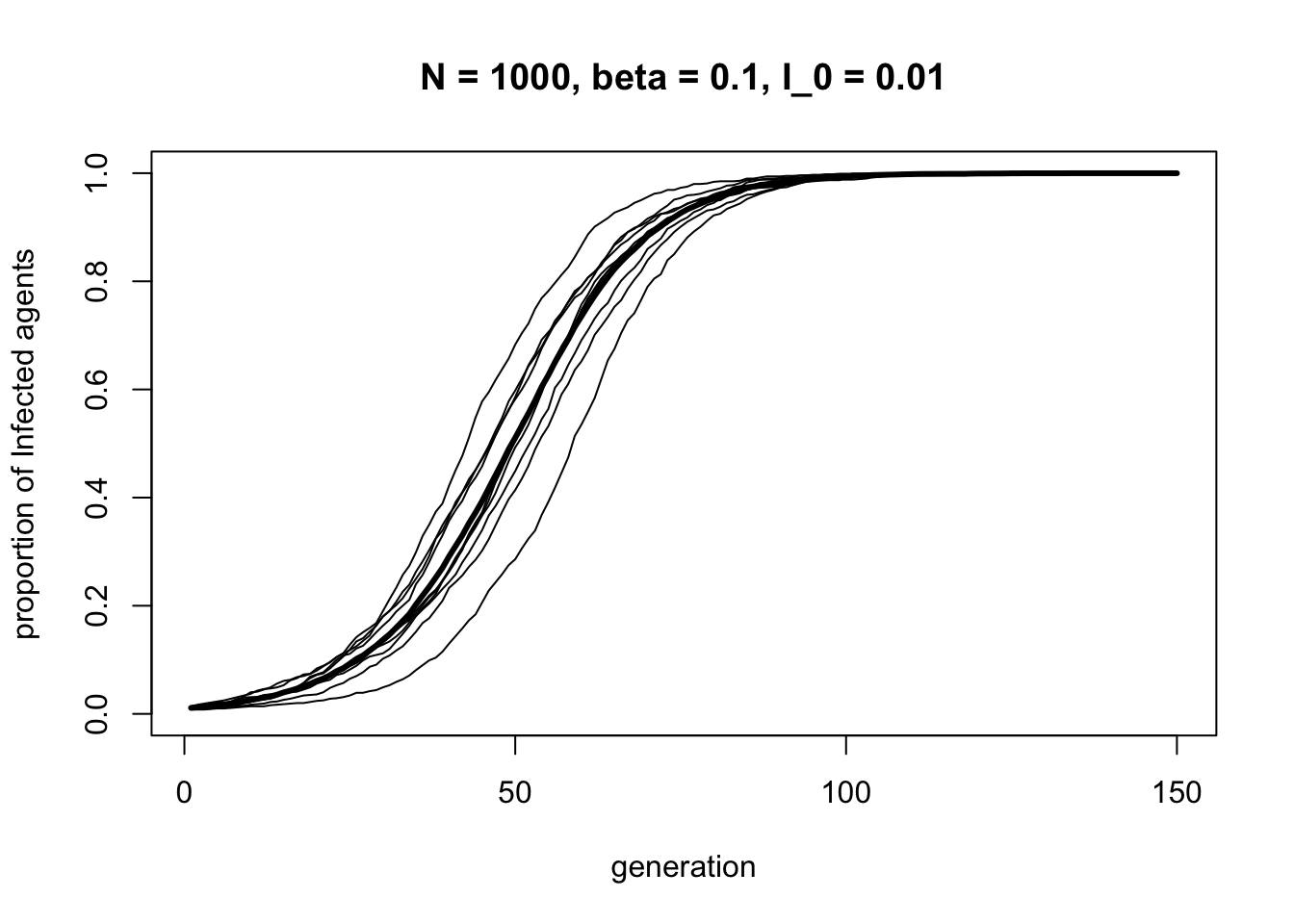
The SI process generates an S-shaped curve. Infections start off slowly, then increase rapidly, then level off as the entire population becomes Infected.
If this function and result looks familiar, it is because it is almost identical to the directly biased cultural transmission implemented in Model 3. Where Model 3 had traits \(A\) and \(B\), here we have \(I\) and \(S\). The strength of biased transmission \(s\) in Model 3 is equivalent to the transmissability parameter \(\beta\) here. It’s the same process. This nicely illustrates one useful function of models: without modelling the two processes, we might not have realised that the two fields were talking about the same process, just with different notation and terminology.
Model 13b: The SIR model
The most common contagion model in epidemiology is the SIR model, which adds a third compartment of Recovered agents. As before, Susceptible agents become Infected with probability \(\beta\), but now Infected agents Recover with probability \(\gamma\). The latter is an asocial process: unlike infection, recovery does not require contact with any other individual to occur. Recovered individuals cannot become Infected again, assuming to have gained immunity.
This is where we should be careful with the disease-idea analogy. While most diseases can be recovered from and be developed immunity to, the same cannot be said for most cultural traits. The best analogy might be with strong religious beliefs (and at the extreme, religious cults), which people join, sometimes leave, and never return to.
The following function adds some code to SImodel specifying that \(I\) individuals become \(R\) with probability \(\gamma\). We now track the frequency of both \(I\) and \(R\) individuals, and plot all three types (the frequency of \(S\) is one minus the frequencies of the other two types, so no need to track that too).
SIRmodel <- function(N, beta, gamma, I_0, t_max, r_max) {

  # create a matrix with t_max rows and r_max columns, fill with NAs, convert to dataframe
  output_I <- as.data.frame(matrix(NA, t_max, r_max))
  output_R <- as.data.frame(matrix(NA, t_max, r_max))

  # purely cosmetic: rename the columns with run1, run2 etc.
  names(output_I) <- paste("run", 1:r_max, sep="")
  names(output_R) <- paste("run", 1:r_max, sep="")

  for (r in 1:r_max) {

    # create first generation
    agent <- data.frame(trait = sample(c("I","S"), N, replace = TRUE,
                                     prob = c(I_0,1-I_0)))

    # add first generation's frequency of I/R to first row of column r
    output_I[1,r] <- sum(agent$trait == "I") / N
    output_R[1,r] <- sum(agent$trait == "R") / N

    for (t in 2:t_max) {

      # 1. biased transmission S to I

      # copy agent to previous_agent dataframe
      previous_agent <- agent

      # for each agent, pick a random agent from the previous generation
      # as demonstrator and store their trait
      demonstrator_trait <- sample(previous_agent$trait, N, replace = TRUE)

      # get N random numbers each between 0 and 1
      copy <- runif(N)

      # # if agent is S, demonstrator is I and with probability beta, acquire I
      agent$trait[previous_agent$trait == "S" &
                  demonstrator_trait == "I" &
                  copy < beta] <- "I"


      # 2. biased mutation I to R

      # copy agent to previous_agent dataframe
      previous_agent <- agent

      # get N random numbers each between 0 and 1
      mutate <- runif(N)

      # if agent was I, with prob gamma, flip to R
      agent$trait[previous_agent$trait == "I" & mutate < gamma] <- "R"


      # get frequency of I/R and put it into output slot for this generation t and run r
      output_I[t,r] <- sum(agent$trait == "I") / N
      output_R[t,r] <- sum(agent$trait == "R") / N

    }

  }

  # first plot a thick line for the mean proportion of I
  plot(rowMeans(output_I),
       type = 'l',
       ylab = "proportion of agents",
       xlab = "generation",
       ylim = c(0,1),
       lwd = 3,
       col = "orange",
       main = paste("N = ", N,
                    ", beta = ", beta,
                    ", gamma = ", gamma,
                    ", I_0 = ", I_0,
                    sep = ""))

  # add lines for R and S
  lines(rowMeans(output_R),
        type = 'l',
        lwd = 3,
        col = "royalblue")

  lines(1 - rowMeans(output_R) - rowMeans(output_I),
        type = 'l',
        lwd = 3,
        col = "grey")

  # add legend
  legend("right",
         legend = c("Susceptible",
                    "Infected",
                    "Recovered"),
         lty = 1,
         lwd = 3,
         col = c("grey", "orange", "royalblue"),
         bty = "n")

  list(output_I = output_I, output_R = output_R)  # export data from function

}
Here is one representative run of the SIR model:
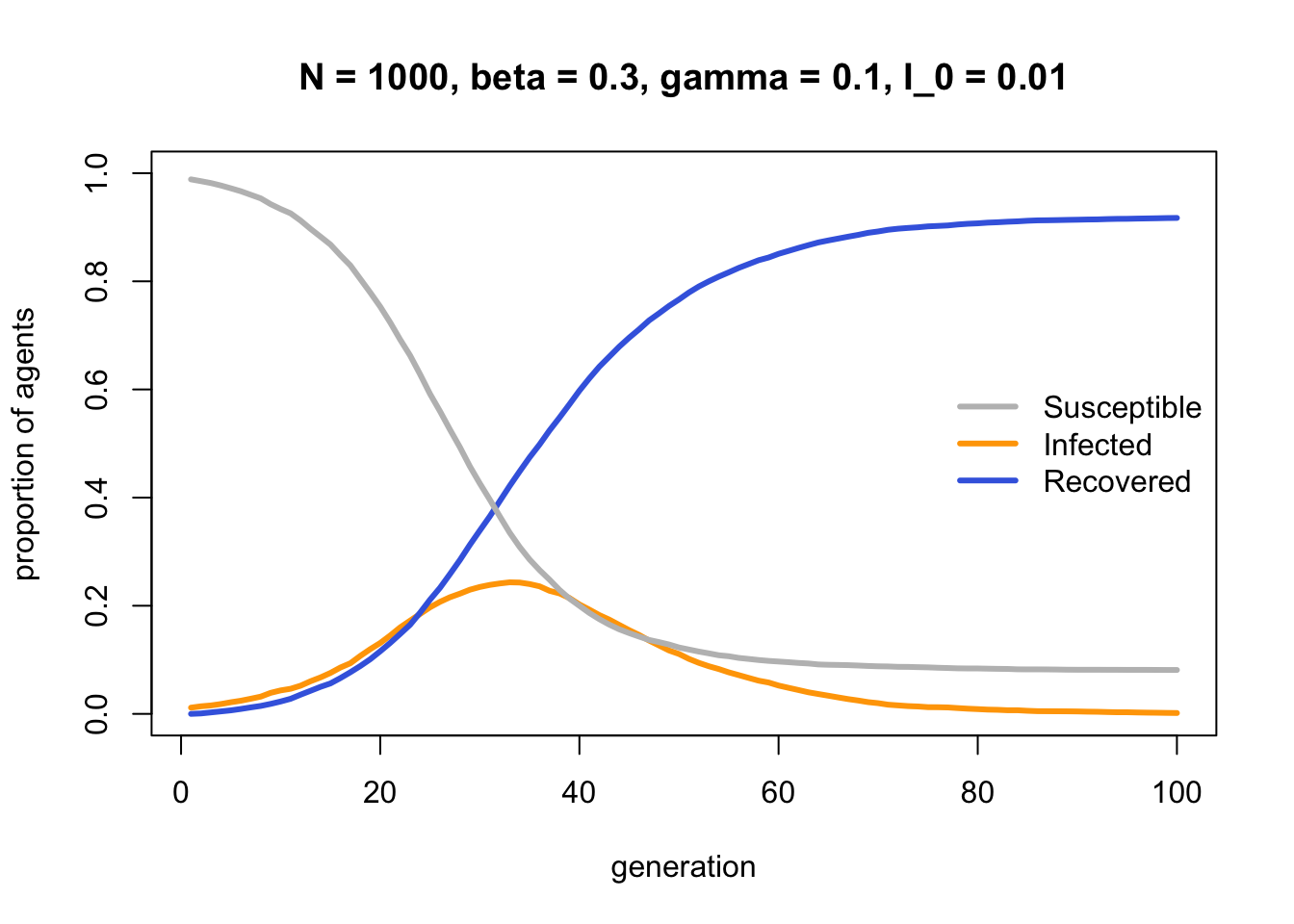
Susceptible agents gradually become Infected, then Infected agents become Recovered. The end state is where every agent is either Susceptible or Recovered, with no Infecteds left to infect any remaining Susceptibles.
As hinted in the SIRmodel comments, the process by which Infected agents become Recovered is identical to biased mutation as seen in Model 2b. Both are individual-level processes occurring independently of other agents. The parameter \(\gamma\) in Model 13b is equivalent to \(\mu_b\) in Model 2b. To confirm this, we can set \(I_0 = 0.99\) and see how \(\gamma\) alone changes the frequency of \(I\):
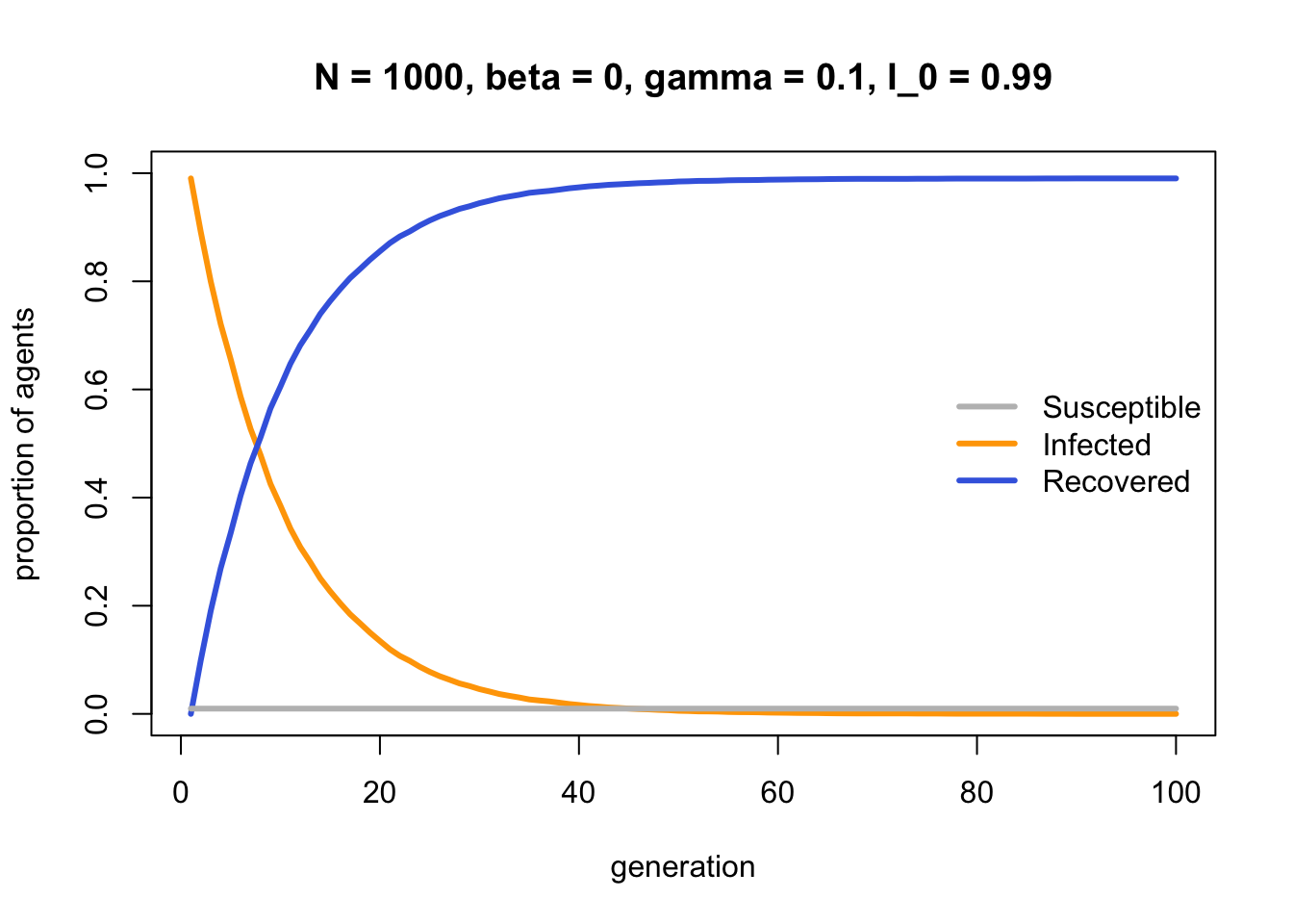
Just as in Model 2b, \(\gamma\) generates an r-shaped diffusion curve, in contrast to the S-shaped curve seen in SImodel above and biased transmission in Model 3.
Model 13c: The SIS model
The SIS model involves Susceptible individuals becoming Infected, as in the SI model, but now Infected individuals can revert to being Susceptible again. In a disease context, this captures a virus like the common cold that one can catch repeatedly. In a social context, it captures cultural traits like jogging or vegetarianism that one might adopt then abandon then adopt again several times during one’s life.
The following function SISmodel is a combination of SImodel and SIRmodel, with biased transmission favouring a switch from \(S\) to \(I\) according to \(\beta\), and biased mutation favouring a switch from \(I\) to \(S\) according to parameter \(\alpha\).
SISmodel <- function(N, beta, alpha, I_0, t_max, r_max) {

  # create a matrix with t_max rows and r_max columns, fill with NAs, convert to dataframe
  output <- as.data.frame(matrix(NA, t_max, r_max))

  # purely cosmetic: rename the columns with run1, run2 etc.
  names(output) <- paste("run", 1:r_max, sep="")

  for (r in 1:r_max) {

    # create first generation
    agent <- data.frame(trait = sample(c("I","S"), N, replace = TRUE,
                                     prob = c(I_0,1-I_0)))

    # add first generation's frequency of I to first row of column run
    output[1,r] <- sum(agent$trait == "I") / N

    for (t in 2:t_max) {

      # 1. biased transmission S to I

      # copy agent to previous_agent dataframe
      previous_agent <- agent

      # for each agent, pick a random agent from the previous generation
      # as demonstrator and store their trait
      demonstrator_trait <- sample(previous_agent$trait, N, replace = TRUE)

      # get N random numbers each between 0 and 1
      copy <- runif(N)

      # if agent is S, demonstrator is I and with probability beta, acquire I
      agent$trait[previous_agent$trait == "S" &
                  demonstrator_trait == "I" &
                  copy < beta] <- "I"

      # 2. biased mutation I to S

      # copy agent to previous_agent dataframe
      previous_agent <- agent

      # get N random numbers each between 0 and 1
      mutate <- runif(N)

      # if agent was I, with prob gamma, flip to R
      agent$trait[previous_agent$trait == "I" & mutate < alpha] <- "S"


      # get frequency of I and put it into output slot for this generation t and run r
      output[t,r] <- sum(agent$trait == "I") / N

    }

  }

  # first plot a thick line for the mean proportion of I
  plot(rowMeans(output),
       type = 'l',
       ylab = "proportion of Infected agents",
       xlab = "generation",
       ylim = c(0,1),
       lwd = 3,
       main = paste("N = ", N,
                    ", beta = ", beta,
                    ", alpha = ", alpha,
                    ", I_0 = ", I_0,
                    sep = ""))

  for (r in 1:r_max) {

    # add lines for each run, up to r_max
    lines(output[,r], type = 'l')

  }

  output  # export data from function

}
Here is one run of the SIS model with \(\alpha = 0.05\), half that of \(\beta\):
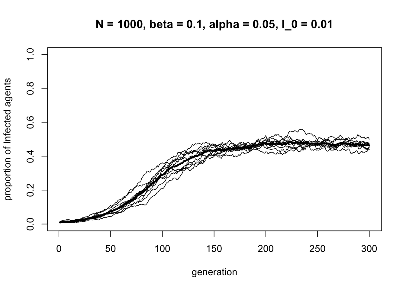
Unlike the previous models, the SIS model produces a stable equilibrium mix of \(S\) and \(I\). This occurs when the number of \(I\)s being converted into \(S\)s equals the number of \(S\)s being converted into \(I\)s. Again, we see how the SIS model can be expressed in terms of cultural evolution concepts from previous models: biased transmission governs the spread of \(I\), whereas biased mutation describes the switch back to \(S\).
Model 13d: The SISa model
Finally, Hill et al. (2010) have proposed the SISa model, which they argue is more representative of social contagion compared to disease contagion. Hill et al. assumed that infection can occur not only via social transmission from others, but also \(a\)socially (or ‘\(a\)utomatically’ as per Hill et al., but asocially makes more sense). People can’t invent diseases, but they can invent new ideas, beliefs, products or technologies, or generally decide to adopt a behaviour independently of anyone else. Hill et al. use the example of obesity, which can be acquired both asocially (deciding not to exercise) and socially (copying the exercise or eating habits of friends).
SISa_model below adds a probability \(a\) that agents mutate from \(S\) to \(I\). We also follow Hill et al. (2010) and add \(n\), the number of demonstrators per timestep that agents potentially learn from during biased transmission of \(S\) to \(I\). This is done by repeating the code implementing biased transmission \(n\) times. With \(n = 1\), this is the same as SISmodel.
SISa_model <- function(N, beta, alpha, a, n, I_0, t_max, r_max) {

  # create a matrix with t_max rows and r_max columns, fill with NAs, convert to dataframe
  output <- as.data.frame(matrix(NA, t_max, r_max))

  # purely cosmetic: rename the columns with run1, run2 etc.
  names(output) <- paste("run", 1:r_max, sep="")

  for (r in 1:r_max) {

    # create first generation
    agent <- data.frame(trait = sample(c("I","S"), N, replace = TRUE,
                                     prob = c(I_0,1-I_0)))

    # add first generation's frequency of I to first row of column run
    output[1,r] <- sum(agent$trait == "I") / N

    for (t in 2:t_max) {

      # 1. biased transmission S to I

      # copy agent to previous_agent dataframe
      previous_agent <- agent

      # for n demonstrators
      for (i in 1:n) {

        # for each agent, pick a random agent from the previous generation
        # as demonstrator and store their trait
        demonstrator_trait <- sample(previous_agent$trait, N, replace = TRUE)

        # get N random numbers each between 0 and 1
        copy <- runif(N)

        # if agent is S, demonstrator is I and with probability beta, acquire I
        agent$trait[previous_agent$trait == "S" &
                    demonstrator_trait == "I" &
                    copy < beta] <- "I"

      }

      # 2. biased mutation I to S

      # copy agent to previous_agent dataframe
      previous_agent <- agent

      # get N random numbers each between 0 and 1
      mutate <- runif(N)

      # if agent was I, with prob gamma, flip to R
      agent$trait[previous_agent$trait == "I" & mutate < alpha] <- "S"


      # 3. biased mutation S to I

      # copy agent to previous_agent dataframe
      previous_agent <- agent

      # get N random numbers each between 0 and 1
      mutate <- runif(N)

      # if agent was S, with prob a, flip to I
      agent$trait[previous_agent$trait == "S" & mutate < a] <- "I"


      # get frequency of I and put it into output slot for this generation t and run r
      output[t,r] <- sum(agent$trait == "I") / N

    }

  }

  # first plot a thick line for the mean proportion of I
  plot(rowMeans(output),
       type = 'l',
       ylab = "proportion of Infected agents",
       xlab = "generation",
       ylim = c(0,1),
       lwd = 3,
       main = paste("N = ", N,
                    ", beta = ", beta,
                    ", alpha = ", alpha,
                    ", a = ", a,
                    ", I_0 = ", I_0,
                    sep = ""))

  for (r in 1:r_max) {

    # add lines for each run, up to r_max
    lines(output[,r], type = 'l')

  }

  output  # export data from function

}
And one run of the SISa model:
data_model13d <- SISa_model(N = 1000,
                            beta = 0.1,
                            alpha = 0.05,
                            a = 0.05,
                            n = 1,
                            I_0 = 0.01,
                            t_max = 100,
                            r_max = 10)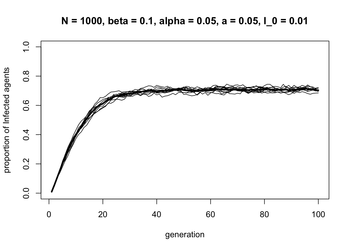
Compared to the SIS model, the SISa model generates a higher equilibrium frequency of \(I\) agents, and reaches this equilibrium faster, due to the addition of mutation from \(S\) to \(I\). The diffusion is also more r-shaped than S-shaped, reflecting the greater role of mutation.
Summary
Social contagion models apply models of disease contagion from epidemiology to culturally transmitted behavioural traits. Naive individuals lacking the trait are Susceptible to becoming Infected with (i.e. socially learning) the trait. Different models provide additional assumptions: SIR models assume individuals can Recover, no longer bearing the trait nor able to learn it again; SIS models assume individuals can revert to being Susceptible after Infection and thus subsequently re-acquire the trait; SISa models assume individuals can asocially learn the trait as well as copy it from Infected individuals. Each of these fits a different kind of cultural trait.
A key take-away is that social contagion models are identical in their underlying mechanics to some of the cultural evolution models we have already covered in this series. The ‘contagion’ component (from \(S\) to \(I\)) is equivalent to directly biased transmission seen in Model 3. The asocial components (from \(I\) to \(R\) or \(S\) in SIR and SIS, and from \(S\) to \(I\) in SISa) are equivalent to biased mutation seen in Model 2b. The \(A\)s and \(B\)s in those models just need to be replaced with \(I\)s and \(S\)s. One value of modelling is to reveal these parallels, so that researchers from different fields can identify common ground despite different terminologies, better learn from each others’ efforts, and avoid reinventing the wheel.
The ultimate value of any model, including social contagion models, is whether it fits real-world data and allows us to predict future cultural dynamics. Hill et al. (2010) showed that the SISa model adequately describes changes in obesity in the Framingham Heart Study Network, a large, long-term health database. From their data, they estimated \(\beta = 0.005\), \(\alpha = 0.035\), \(a = 0.019\) and \(n = 3\) per year/timestep, for a dataset of \(N = 3500\). We can plug these values into SISa_model to predict what will happen in the long-term, and calculate the expected equilibrium frequency of obesity:
data_model13d <- SISa_model(N = 3500,
                            beta = 0.005,
                            alpha = 0.035,
                            a = 0.019,
                            n = 3,
                            I_0 = 0.01,
                            t_max = 150,
                            r_max = 10)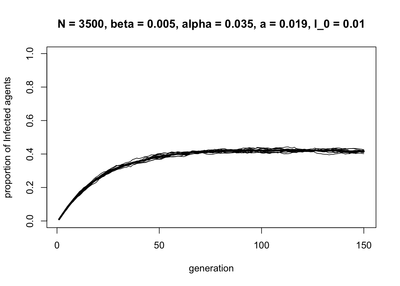
##       150
## 0.4181429
This recreates Hill et al.’s (2010) Figure 5A. The actual rate of obesity in the Framingham sample was 14% in the 1970s and 30% in 2000. This model predicts that obesity will eventually reach an equilibrium frequency of 42%. As Hill et al. remark, “While not great, this is a much more optimistic estimate than 100%”. They also show that, despite \(\beta\) being smaller than \(\gamma\) and \(a\), changing \(\beta\) has a larger effect on decreasing obesity per unit decrease in rate than the other parameters. This suggests that interventions aimed at reducing the social transmission of obesity will be more effective than interventions focused on asocial factors.
Other work has extended contagion models to further suit a cultural, rather than disease, context. Bettencourt et al. (2006) proposed and analysed an SEIZ model, where Susceptible individuals become Exposed (\(E\)) to an idea before eventually either becoming Infected (i.e. adopting it), or rejecting it (\(Z\)). They showed that this SEIZ model better captures the spread of the use of Feynman diagrams amongst post-war physicists, compared to simpler models lacking either \(E\) or \(Z\) classes. Walters & Kendal (2013), meanwhile, adapted an SIS model to make the social transmission from \(S\) to \(I\) conformist (see Model 5) rather than directly biased, with possible applications to the spread of binge drinking.
Exercises
Make a list of cultural traits that might be suitably described by the four different models implemented above (SI, SIR, SIS and SISa). How else might you modify the basic SI model to better suit the dynamics of other cultural traits not in any of your lists?
The SISa model assumes biased transmission from \(S\) to \(I\), and biased mutation of both \(S\) and \(I\). In theory, biased transmission could also drive the switch from \(I\) back to \(S\). For example, one might copy the healthy eating or exercise habits of a friend to lose weight and no longer be obese. Add this biased transmission to SISa_model. Explore the dynamics generated by varying the four parameters (\(\beta\), \(\alpha\), \(a\) and your new parameter).
Following Walters & Kendal (2013), and using code from Model 5, replace the directly biased social learning of SISmodel with conformist social learning. Explore how increasing the conformity parameter \(D\) affects the equilibrium value of \(I\).
References
Anderson, R. M., & May, R. M. (1992). Infectious diseases of humans: dynamics and control. Oxford University Press.
Bettencourt, L. M., Cintrón-Arias, A., Kaiser, D. I., & Castillo-Chávez, C. (2006). The power of a good idea: Quantitative modeling of the spread of ideas from epidemiological models. Physica A, 364, 513-536.
Hill, A. L., Rand, D. G., Nowak, M. A., & Christakis, N. A. (2010). Infectious disease modeling of social contagion in networks. PLOS Computational Biology, 6(11), e1000968.
Walters, C. E., & Kendal, J. R. (2013). An SIS model for cultural trait transmission with conformity bias. Theoretical Population Biology, 90, 56-63.