Model 16: Bayesian iterated learning
Introduction
Model 16 covers a slightly different approach to cultural evolution compared to the population-genetic-inspired models covered previously. These models draw instead from cognitive science, statistics and linguistics. They use the statistical tools of Bayesian inference to explore how cognitive representations or linguistic features evolve over time as they are passed from person to person, generation to generation. After introducing the concepts of Bayesian inference and iterated learning, Model 16 concerns the emergence of regularisation in language evolution.
Bayesian inference
Bayesian inference is a statistical approach to the problem of how to update one’s beliefs in light of new data. Let’s use an example to illustrate this, inspired by Perfors et al. (2011). Imagine that you develop a headache. This is the data you receive from the world, in this case from your body. Assume for the purposes of this simple example that you can only think of three possible causes for the headache: dehydration, a brain tumour, and indigestion. These are your hypotheses. Bayesian induction involves combining the likelihood of observing the data given each hypothesis with your prior beliefs about those hypotheses to generate posterior probabilities for each hypothesis, given the new data.
Likelihoods are denoted \(P(d|h_i)\), which means the probability of the data \(d\) given hypothesis \(h_i\). Given that both dehydration and brain tumours are highly likely to cause headaches while indigestion is not, we set our likelihoods as \(P(d|h_{dehydration} = 0.9)\), \(P(d|h_{tumour} = 0.8)\) and \(P(d|h_{indigestion} = 0.1)\). (Note that these probabilities do not have to be explicitly or consciously held by anyone, they just represent people’s estimates for modelling purposes without worrying about how they are implemented mechanistically in the brain. We do not need to assume that people are explicitly calculating Bayes’ rule for Bayesian inference to be a good approximation of human decision making.) Priors, denoted \(P(h_i)\), represent your estimate of the probability of each hypothesis before seeing any data. Because you often suffer from dehydration and indigestion, but have never had a brain tumour and which you know are (thankfully) rare in the population, your priors are \(P(h_{dehydration} = 0.4)\), \(P(h_{tumour} = 0.1)\) and \(P(h_{indigestion} = 0.5)\). Note that these prior probabilities sum to one, because this is the full set of hypotheses that we are considering, and one of them must be responsible for the headache.
The posterior probabilities of each hypothesis \(h_i\) given the data, denoted \(P(h_i|d)\), are then given by Bayes’ rule:
\[P(h_i|d) = \frac{ P(d|h_i) P(h_i) } { \sum_{h_j \in H}{ P(d|h_j) P(h_j)} } \]
Bayes’ rule says that the posterior probability of hypothesis \(h_i\) is equal to its likelihood multiplied by its prior probability. The denominator is simply the sum of the posterior probabilities for the set of all hypotheses (denoted \(H\)) and ensures that all posterior probabilities sum to one. Plugging in our hypothetical likelihoods and priors from above, we have:
\[ P(h_{dehydration}|d) = \frac{ 0.9 * 0.4 } { (0.9 * 0.4) + (0.8 * 0.1) + (0.1 * 0.5) } = 0.735 \] \[ P(h_{tumour}|d) = \frac{ 0.8 * 0.1 } { (0.9 * 0.4) + (0.8 * 0.1) + (0.1 * 0.5) } = 0.163 \] \[ P(h_{indigestion}|d) = \frac{ 0.1 * 0.5 } { (0.9 * 0.4) + (0.8 * 0.1) + (0.1 * 0.5) } = 0.102 \]
Bayesian inference tells us that dehydration is a far more likely cause of our headache than either a brain tumour or indigestion. This is probably the conclusion you reached at the very beginning - obviously dehydration is the most likely explanation! That’s good, as it indicates that a Bayesian approach adequately approximates your intuitive judgements. However, intuitions can’t be put directly into a model, and Bayesian inference provides one way of quantifying how people balance the likelihood of explanations with their prior beliefs to reach a judgement. It’s also useful for modelling more complex cases than our simple example which have more data and a larger hypothesis space, such as learning languages, as we will see later. Finally, unlike other approaches, Bayesian inference is useful because it is probabilistic rather than all-or-nothing. We do not seek to accept or reject hypotheses, rather we seek a probability distribution across all possible hypotheses to estimate our (un)certainty in each one.
Iterated learning
Iterated learning is the name given by some cognitive scientists (e.g. Griffiths et al. 2008) and linguists (e.g. Smith & Kirby 2008) to describe the repeated transmission of information from individual to individual along a linear chain of learners. This is much like the ‘transmission chains’ discussed previously that have been used to study transmission biases in the lab. However, iterated learning is usually placed within a Bayesian framework. The data \(d\) comes not from the physical world, nor one’s own body (as in the headache example above), but from other individuals. Specifically, each individual in the chain generates some data \(d\) which is observed by the next individual in the chain. Each learner combines their priors with the likelihood of the culturally-transmitted data using Bayes’ rule, to generate a posterior distribution across all potential hypotheses. This posterior is used to generate new data which is passed to the next individual in the chain, and so on along the chain.
Linguists have used iterated learning to study language evolution (e.g. Kirby et al. 2007; Smith & Kirby 2008). Here the data are utterances that contain information about vocabulary or grammatical rules. Subsequent language learners, such as infants learning their first language or adults learning a second language, must infer the grammatical rules of the language from the limited data they receive from other speakers. The priors in this context are innate, cognitively attractive or culturally acquired expectations about the possible hypothesis space of real languages. Cognitive scientists have used Bayesian iterated learning to address similar questions for non-linguistic culturally transmitted representations, such as object categorisation schemes or colour terminologies (e.g. Griffiths et al. 2008). The question addressed by all this research, as well as Model 16, is: how do languages or cognitive representations culturally evolve over time under the assumption of Bayesian iterated learning? One major claim that we will examine in these models is that languages and cognitive structures always come to reflect the priors (or ‘inductive biases’) of the learners, irrespective of the initial data observed by the first individual in the chain.
Model 16
Model 16 recreates a common model of Bayesian iterated learning examining the emergence of linguistic regularisation, as developed by Reali & Griffiths (2009), Ferdinand et al. (2014) and Navarro et al. (2018), amongst others. As always, this model is highly simplified compared to real languages and language learning. But as we have repeatedly seen, simple models are useful for understanding such complex phenomena precisely because of their simplicity.
Imagine a grammatical feature that can take one of two forms. For example, verbs can either follow the subject (“I go”) or precede the subject (“go I”). (NB While I use a linguistic example here, technically this model applies to any socially transmitted trait that takes two forms, e.g. social conventions such as shaking hands with either the right or the left hand.) We define \(\theta\) as the probability of one variant (say, subject-verb) being used in the language, and \(1 - \theta\) as the probability of the other variant (verb-subject) being used. Your task as a naive learner is to infer from a set of utterances the grammatical rule used in your society, i.e. to infer the value of \(\theta\) for this language, which is unknown to you except via data received from other speakers.
In particular, we are interested in whether the language is regular or irregular. A regular language always uses the same variant (e.g. always subject-verb, or always verb-subject). Regular languages therefore have either \(\theta = 0\) or \(\theta = 1\). An irregular language uses some mix of variants (e.g. sometimes subject-verb, sometimes verb-subject). Irregular languages therefore have \(0 < \theta < 1\). A highly irregular language has \(\theta \approx 0.5\), such that one variant is used about half the time and the other variant used the other half.
Our hypothesis space is therefore the full range of possible \(\theta\) values. Because \(\theta\) is a probability, this goes from 0 to 1 on a continuous scale. We will call this hypothesis space \(p\) and code it as follows:
##   [1] 0.00 0.01 0.02 0.03 0.04 0.05 0.06 0.07 0.08 0.09 0.10 0.11 0.12 0.13 0.14
##  [16] 0.15 0.16 0.17 0.18 0.19 0.20 0.21 0.22 0.23 0.24 0.25 0.26 0.27 0.28 0.29
##  [31] 0.30 0.31 0.32 0.33 0.34 0.35 0.36 0.37 0.38 0.39 0.40 0.41 0.42 0.43 0.44
##  [46] 0.45 0.46 0.47 0.48 0.49 0.50 0.51 0.52 0.53 0.54 0.55 0.56 0.57 0.58 0.59
##  [61] 0.60 0.61 0.62 0.63 0.64 0.65 0.66 0.67 0.68 0.69 0.70 0.71 0.72 0.73 0.74
##  [76] 0.75 0.76 0.77 0.78 0.79 0.80 0.81 0.82 0.83 0.84 0.85 0.86 0.87 0.88 0.89
##  [91] 0.90 0.91 0.92 0.93 0.94 0.95 0.96 0.97 0.98 0.99 1.00
The granularity here is somewhat arbitrary. I’ve chosen intervals of 0.01, but you could use a smaller interval to get a more fine-grained hypothesis space and therefore more accurate results, albeit at the cost of longer run times.
The data take the form of \(n\) independent observations of the grammatical rule. In the context of an iterated learning chain, this is like hearing \(n\) examples of the grammatical rule from the previous individual in the chain. We assume that \(k\) of these observations fit variant 1 (e.g. subject-verb) while \(n - k\) fit variant 2 (e.g. verb-subject). In our simulations we will assume \(n = 10\) observations with \(k = 5\) of those fitting the first variant:
Note that while \(p\) is a continuous probability ranging from 0 to 1, \(k\) is an integer that varies from 0 to \(n\). Our initial \(k\) implies a highly irregular language, given that half of the utterances fit variant 1 (e.g. subject-verb) and half fit variant 2 (e.g. verb-subject). However, this is a very small set of data, and may not accurately reflect the \(\theta\) of the entire language. A \(\theta\) of 0.5 could generate \(k = 5\), but so could a range of other \(\theta\) values. Conversely, \(\theta = 0.5\) won’t always generate 5/10 observations, just as flipping a coin 10 times doesn’t always give 5 heads and 5 tails. This is where Bayesian inference comes in: we must infer \(\theta\) from the likelihood of our data, as well as our priors.
First the likelihoods. The likelihood of \(k\) successes in \(n\) independent events with two outcomes, success/fail, is given by the binomial distribution. In our case a ‘success’ is an observation of grammatical variant 1 and a ‘fail’ is an observation of variant 2. The likelihoods for our data across all possible hypotheses in \(p\) can be obtained using the dbinom command:
lik <- dbinom(k, n, p)

plot(lik,
     x = p,
     xlab = expression(theta),
     ylab = "",
     type = 'l',
     main = "likelihood for k = 5, n = 10")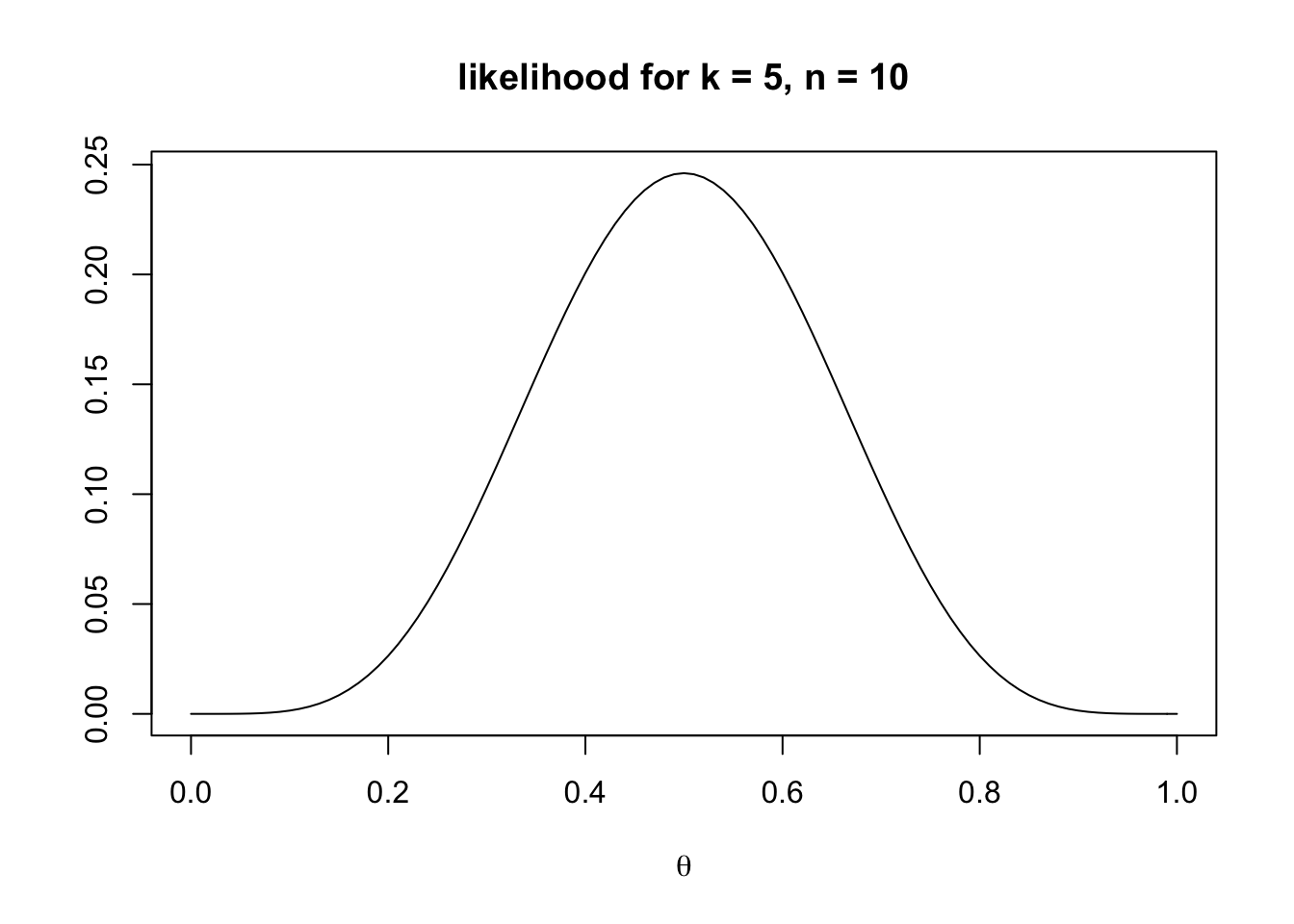
The plot shows, as we would expect, that a \(\theta\) of 0.5 most likely generates \(k = 5\) observations, but that a range of other values are also possible. Try different values of \(k\) to see how the likelihoods change.
Now the priors. Reali & Griffiths (2009) introduced the beta distribution for quantifying priors in this regularisation model. The beta distribution takes two parameters that determine its shape, \(\alpha\) and \(\beta\). For now we will assume \(\alpha = \beta\) so we have one less parameter to worry about. Assuming \(\alpha = \beta\) also gives symmetrical distributions which are easier to interpret. The following code shows a beta distribution with \(\alpha = 1\):
alpha <- 1
beta <- alpha

prior <- dbeta(p, alpha, beta)

plot(prior,
     x = p,
     xlab = expression(theta),
     ylab = "",
     type = 'l',
     main = "flat prior (alpha = 1)")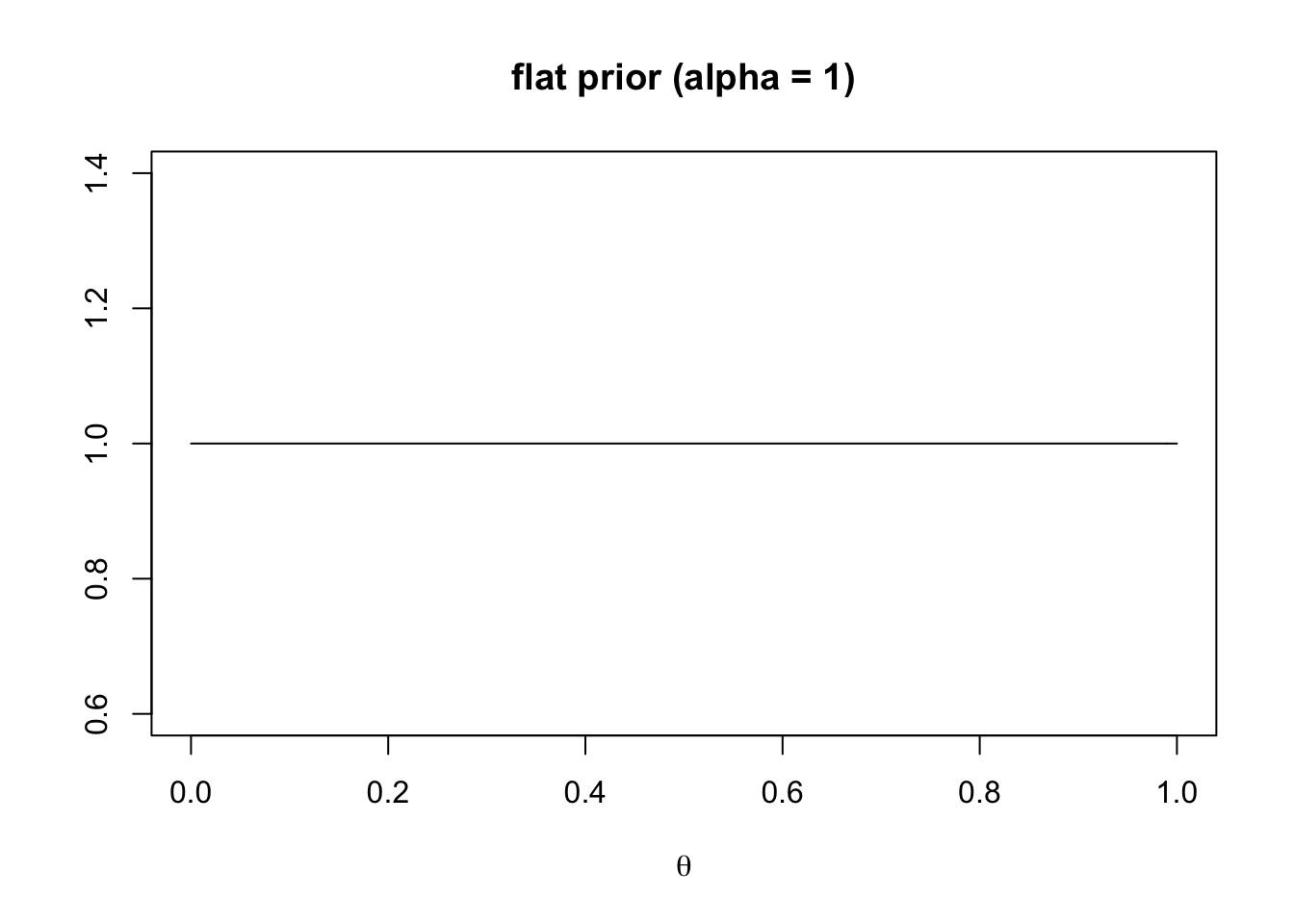
This gives a flat prior. The learner expects every value of \(\theta\) to be equally likely and brings no particular expectation to the inference problem.
Reducing \(\alpha\) to less than 1 gives a prior distribution concentrated at 0 and 1:
alpha <- 0.1
beta <- alpha

prior <- dbeta(p, alpha, beta)

plot(prior,
     x = p,
     xlab = expression(theta),
     ylab = "",
     type = 'l',
     main = "regularisation prior (alpha = 0.1)")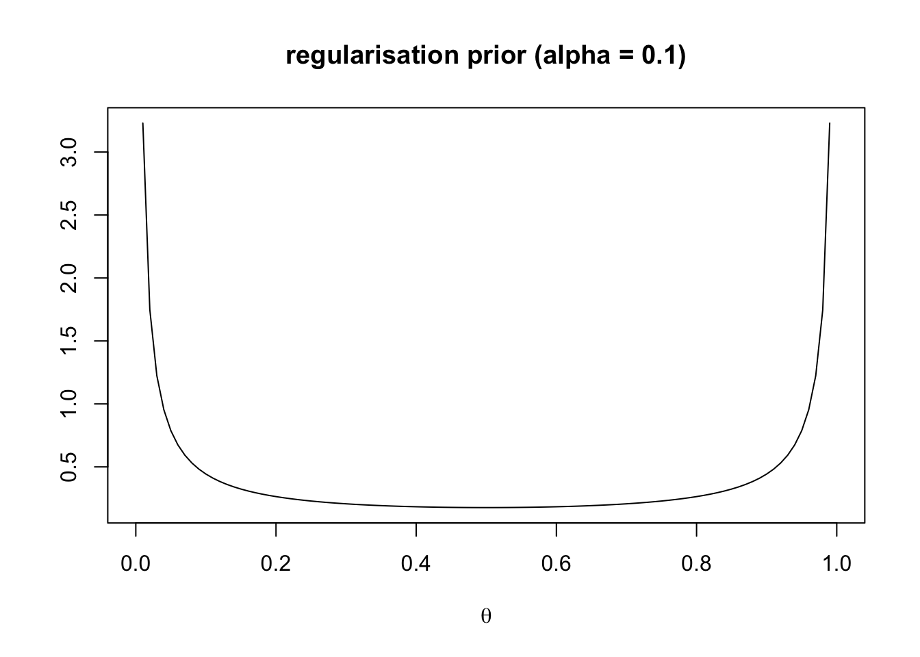
This represents a regularisation prior. The learner expects a regular language, i.e. one which either always has feature 1 (\(\theta = 1\)) or always has feature 2 (\(\theta = 0\)).
Finally, increasing \(\alpha\) above 1 generates a bell-shaped distribution much like a normal distribution:
alpha <- 5
beta <- alpha

prior <- dbeta(p, alpha, beta)

plot(prior,
     x = p,
     xlab = expression(theta),
     ylab = "",
     type = 'l',
     main = "irregularisation prior (alpha = 5)")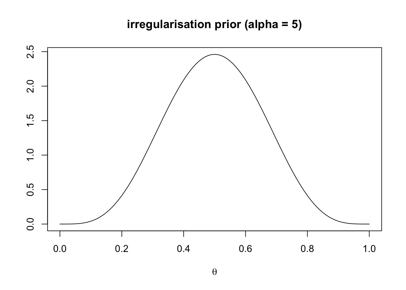
This represents an irregularisation prior. The learner expects an irregular language with a \(\theta\) peaking at 0.5, meaning that both grammatical variants are equally likely to be observed in the language.
The posterior distribution is then obtained by multiplying the likelihood by the prior and dividing by the sum of all posterior probabilities, as per Bayes’ rule. The following code does this for the flat priors:
alpha <- 1
beta <- alpha

prior <- dbeta(p, alpha, beta)

post <- lik*prior
post <- post / sum(post)

plot(post,
     x = p,
     xlab = expression(theta),
     ylab = "",
     type = 'l',
     main = "posterior for flat prior")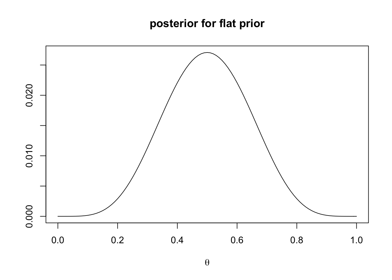
With a flat prior, the posterior is entirely determined by the likelihood and centres on \(\theta = 0.5\), just like the likelihood. What about a regularisation prior?
alpha <- 0.1
beta <- alpha

prior <- dbeta(p, alpha, beta)

post <- lik*prior
post <- post / sum(post, na.rm = TRUE)

plot(post,
     x = p,
     xlab = expression(theta),
     ylab = "",
     type = 'l',
     main = "posterior for regularisation prior")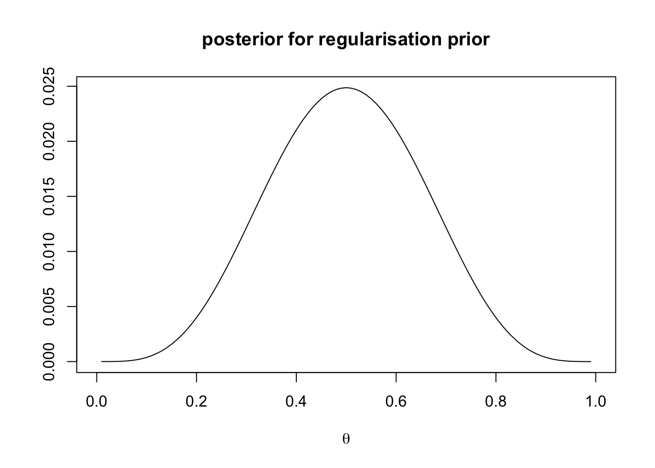
Here the prior seems to have very little effect on the posterior distribution, which again looks very similar to the likelihood.
Finally irregularisation priors:
alpha <- 5
beta <- alpha

prior <- dbeta(p, alpha, beta)

post <- lik*prior
post <- post / sum(post)

plot(post,
     x = p,
     xlab = expression(theta),
     ylab = "",
     type = 'l',
     main = "posterior for irregularisation prior")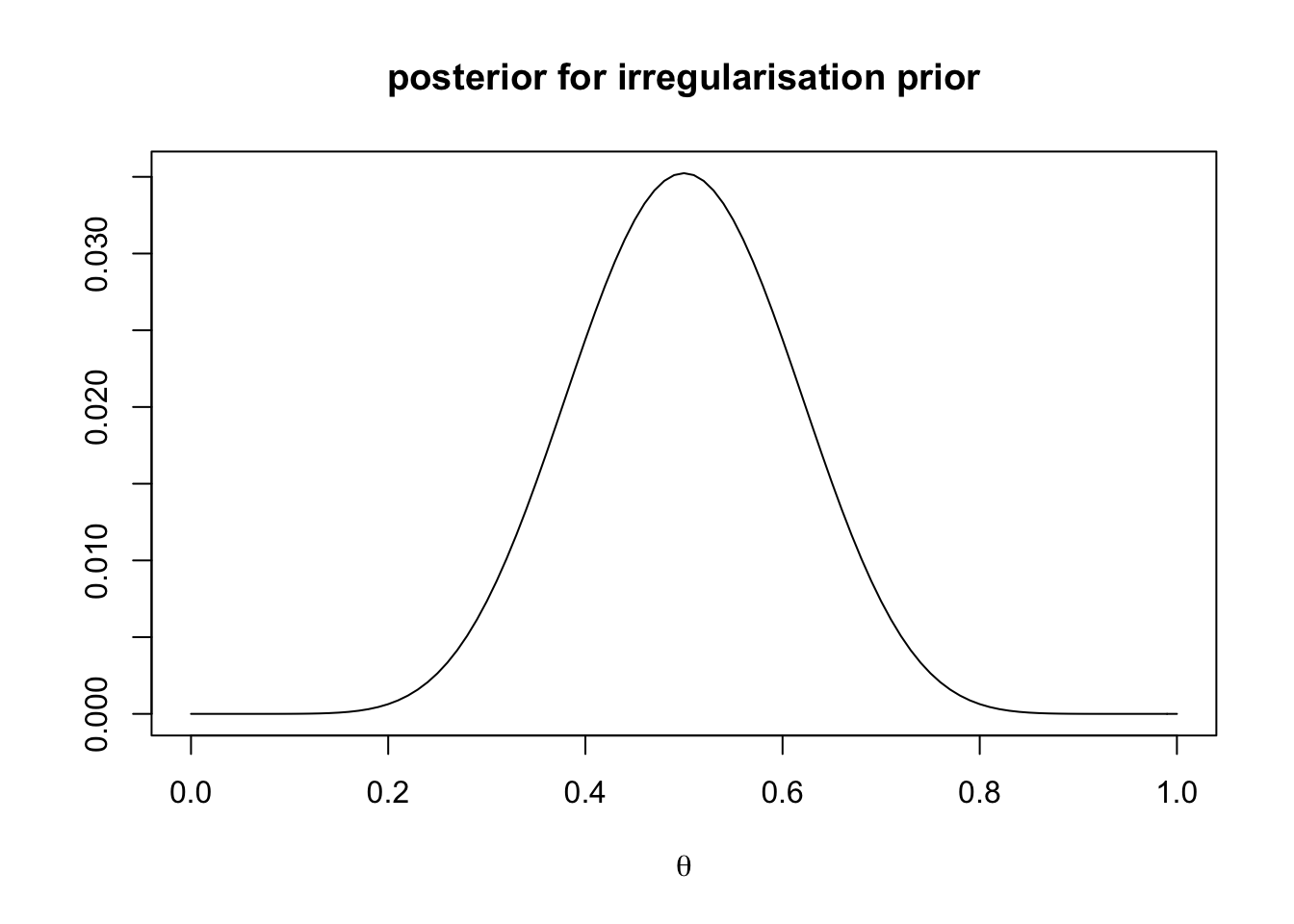
Because the prior and likelihood agree in this case, the posterior looks narrower than either of them. Our confidence in \(\theta = 0.5\) has increased. Try different values of \(k\) and \(\alpha\) to explore how priors and likelihoods combine to generate posterior distributions.
Before going further, we can take advantage of a Bayesian trick to simplify and speed up our code. A binomial likelihood and a beta prior form what is known as a conjugate pair. The posterior distribution of such a pair is a beta distribution with parameters \(k + \alpha\) and \(n - k + \beta\). Don’t worry about the details or derivation of this, it’s best to just take it as a statistical convenience. The key thing is that we can use this fact to generate the posterior direct from \(k\), \(\alpha\) and \(\beta\), without having to calculate the prior and likelihood and multiply them together. Let’s compare the new conjugate method with the old step-by-step method:
# old method
lik <- dbinom(k, n, p)
prior <- dbeta(p, alpha, beta)

post <- lik*prior
post <- post / sum(post)

head(post)
## [1] 0.000000e+00 8.438890e-15 3.943421e-12 1.382310e-10 1.677064e-09
## [6] 1.137132e-08# new method
post_conjugate <- dbeta(p, k + alpha, n - k + beta)
post_conjugate <- post_conjugate / sum(post_conjugate)
head(post_conjugate)## [1] 0.000000e+00 8.438890e-15 3.943421e-12 1.382310e-10 1.677064e-09
## [6] 1.137132e-08I only show the first six values using head() for brevity, but you can see that they are identical. You can check yourself that the rest is identical. We’ll use this more efficient method from now on.
So far we have generated a posterior distribution from some data. In an iterated learning chain, this occurs when an individual receives data from the previous individual in the chain. Now we need to simulate the next step, where this receiving individual generates new data from their posterior distribution to pass on to the next individual in the chain.
First we need to pick a value of \(\theta\) from the posterior distribution. This will be the hypothesis used to generate the data.
There are two ways of doing this. The first is to randomly sample from the hypothesis space in proportion to the posterior probabilities. This is known as ‘sampling’. Now that we know the conjugate shortcut to calculating the posterior, this can be done with a single rbeta command:
## [1] 0.6486422\(\theta\) here should be close to 0.5, but not exactly 0.5 because we are randomly sampling.
The second way of choosing a \(\theta\) is to pick the hypothesis with the maximum posterior probability. This is known as the ‘maximum a posteriori’ (MAP) hypothesis. To obtain this we can use the formulae for the mode of a beta distribution (you can look this up on wikipedia):
if ((k + alpha) > 1 & (n - k + beta) > 1) {

  theta <- (k + alpha - 1) / (n + alpha + beta - 2)

} else if ((k + alpha) <= 1 & (n - k + beta) > 1) {

  theta <- 0

} else if ((k + alpha) > 1 & (n - k + beta) <= 1) {

  theta <- 1

}

theta
## [1] 0.5\(\theta\) here should be exactly 0.5 given that this is the maximum of this posterior distribution.
Now we need to use our \(\theta\) to generate a new \(k\) to be the data for the next individual in the chain. This is another task for the binomial distribution, which converts probabilities into discrete picks. The following code uses rbinom to pick a random draw from a binomial with \(n\) trials and probability of success \(\theta\):
## [1] 5The new \(k\) should be an integer around 5, but possibly not exactly 5, given that we are sampling from only \(n = 10\) observations.
Finally we can generate a probability distribution for all possible values of \(k\) across all values of \(\theta\). We label this prob_k. You can think of this as the posterior transformed from a continuous probability from 0 to 1 into a discrete integer scale from 0 to \(n\) to give the probability of each new \(k\), without the stochasticity introduced by random picks. The following code cycles through all integers from 0 to \(n\) and, for each one, multiplies the posterior across all \(p\) values by the binomial distribution for that integer (like we did above with the likelihood). We then sum across all \(p\) values and normalise to ensure prob_k sums to 1.
# get probability distribution of new picks
prob_k <- rep(NA, n+1)
names(prob_k) <- 0:n

for (j in 0:n) {

  prob_k[j+1] <- sum( dbinom(j, n, p) * post )

}

prob_k <- prob_k / sum(prob_k)
prob_k
## 0 1 2 3 4 5 6
## 0.00461198 0.02427358 0.06675234 0.12565146 0.17866067 0.20009995 0.17866067
## 7 8 9 10
## 0.12565146 0.06675234 0.02427358 0.00461198As expected, \(k = 5\) is most likely, but other values are also quite likely to be picked too.
Now let’s put all these bits of code into a function, BayesianInference, which takes data \(k\) and the other parameters as input and generates and exports both the new \(k\) value and the entire \(k\) probability distribution. Note (i) we set the default \(\beta\) to be equal to \(\alpha\) so that if \(\beta\) is left unspecified it defaults to be equal to \(\alpha\); (ii) we add a couple of lines of code to avoid infinity in the posterior when the conjugate beta parameters are less than 1; and (iii) we define a variable sampling which implements sampling if TRUE (the default) and MAP if FALSE.
BayesianInference <- function(n = 10,
                              k = 5,
                              alpha = 1,
                              beta = alpha,
                              sampling = TRUE) {

  # hypothesis space
  p <- seq(0, 1, by = 0.01)

  # avoid infinity when beta distribution parameters are less than 1
  if ((k + alpha) < 1) p[1] <- 0.00001
  if ((n - k + beta) < 1) p[length(p)] <- 0.99999

  # generate posterior
  post_conjugate <- dbeta(p, k + alpha, n - k + beta)
  post_conjugate <- post_conjugate / sum(post_conjugate)

  if (sampling == TRUE) {

    # pick a random sample from the posterior
    theta <- rbeta(1, k + alpha, n - k + beta)

  } else {

    # pick the maximum posterior probability (MAP)

    if ((k + alpha) > 1 & (n - k + beta) > 1) {

      theta <- (k + alpha - 1) / (n + alpha + beta - 2)

    } else if ((k + alpha) <= 1 & (n - k + beta) > 1) {

      theta <- 0

    } else if ((k + alpha) > 1 & (n - k + beta) <= 1) {

      theta <- 1

    }

  }

  # draw a new k from a binomial using theta
  k <- rbinom(1, n, theta)

  # get probability distribution of new picks
  prob_k <- rep(NA, n+1)
  names(prob_k) <- 0:n

  for (j in 0:n) {

    prob_k[j+1] <- sum( dbinom(j, n, p) * post_conjugate )

  }

  prob_k <- prob_k / sum(prob_k)

  # export new k and prob_k
  list(k = k, prob_k = prob_k)

}
Here is an example output with regularisation priors:
## $k
## [1] 3
##
## $prob_k
##          0          1          2          3          4          5          6
## 0.01055127 0.03816419 0.07996999 0.12513211 0.15979708 0.17277071 0.15979708
##          7          8          9         10
## 0.12513211 0.07996999 0.03816419 0.01055127
Now we can use BayesianInference to simulate an iterated learning chain of \(N = 20\) individuals. Let’s go step by step. The output will be each agents’ \(k\) and prob_k. These are held in a vector and matrix respectively, initialised with zeroes:
N <- 20

# vector to hold N k values
k_vector <- rep(0, N)

# matrix to hold N probability distributions for k
k_matrix <- matrix(0, nrow = N, ncol = n+1)
For the actual iterated learning, we cycle through \(N\) agents, for each one getting the next generation’s \(k\) and prob_k using BayesianInference. For now we use its default parameters, which specify flat priors (\(\alpha = 1\)). \(k\) and prob_k are stored in k_vector and k_matrix respectively. We also update the current value of \(k\) with the new one to pass to the next generation.
for (i in 1:N) {

  next_gen <- BayesianInference()

  # k for next generation
  k <- next_gen$k

  # store probability distribution and k
  k_vector[i] <- next_gen$k
  k_matrix[i,] <- next_gen$prob_k

}
A look at k_vector reveals a range of values:
## [1] 8 9 5 7 3 2 7 2 5 0 6 5 2 6 3 3 5 6 6 4There is lots of stochasticity here, and ideally we would like to generalise across multiple independent iterated learning chains. Let’s do this by putting the \(N\) loop above inside a loop over \(r_{max} = 10000\) runs. As in previous models, we keep a running total in k_vector and k_matrix and then divide them by \(r_{max}\) at the end to get their mean values across all runs. We also need to reset \(k\) to the initial default value at the start of every run, otherwise each run would start with the last \(k\) of the previous run making them non-independent.
r_max <- 10000
k <- 5

# vector to hold N k values
k_vector <- rep(0, N)

# matrix to hold N probability distributions for k
k_matrix <- matrix(0, nrow = N, ncol = n+1)

# record starting k
k_initial <- k

for (r in 1:r_max) {

  k <- k_initial

  for (i in 1:N) {

    next_gen <- BayesianInference()

    # k for next generation
    k <- next_gen$k

    # store probability distribution and k
    k_vector[i] <- k_vector[i] + next_gen$k
    k_matrix[i,] <- k_matrix[i,] + next_gen$prob_k

  }

}

# average across all runs
k_vector <- k_vector / r_max
k_matrix <- k_matrix / r_max
We can now clearly see that the mean k_vector across all \(r_{max} = 10000\) runs is close to 5, as expected for a flat prior and starting \(k = 5\):
##  [1] 5.0147 5.0178 4.9395 4.9792 4.9872 4.9996 5.0278 4.9957 5.0266 4.9832
## [11] 4.9862 4.9757 4.9797 5.0371 4.9837 5.0049 4.9834 4.9893 4.9847 4.9996
As usual we wrap all this in a function which we call IteratedLearning. Note that we set all the parameter values in the IteratedLearning call and pass them to BayesianInference. We also export the parameters for use later in plotting functions.
IteratedLearning <- function(n = 10,
                             k = 5,
                             alpha = 1,
                             beta = alpha,
                             sampling = TRUE,
                             N = 20,
                             r_max = 10000) {

  # vector to hold N k values
  k_vector <- rep(0, N)

  # matrix to hold N probability distributions for k
  k_matrix <- matrix(0, nrow = N, ncol = n+1)

  # record starting k
  k_initial <- k

  for (r in 1:r_max) {

    # reset k
    k <- k_initial

    for (i in 1:N) {

      next_gen <- BayesianInference(n,
                                    k,
                                    alpha,
                                    beta,
                                    sampling)

      # k for next generation
      k <- next_gen$k

      # store probability distribution and k
      k_vector[i] <- k_vector[i] + next_gen$k
      k_matrix[i,] <- k_matrix[i,] + next_gen$prob_k

    }

  }

  # average across all runs
  k_vector <- k_vector / r_max
  k_matrix <- k_matrix / r_max

  # export k_vector, k_matrix and parameters
  list(k_vector = k_vector,
       k_matrix = k_matrix,
       parameters = c(n = n,
                      k = k_initial,
                      alpha = alpha,
                      beta = beta,
                      sampling = sampling,
                      N = N,
                      r_max = r_max))

}
To verify everything worked as expected we can check that the k_vector from the default values matches the ones shown above.
##  [1] 4.9917 5.0196 5.0153 5.0109 5.0068 5.0037 4.9819 4.9699 4.9654 4.9808
## [11] 4.9928 4.9857 4.9887 4.9993 4.9897 5.0061 5.0257 5.0169 5.0151 5.0323
If you inspect k_vector for \(\alpha = 0.1\), \(\alpha = 1\) and \(\alpha = 5\) you’ll see that they are all around 5. However this mean value obscures different underlying probability distributions. To see this, we can follow Reali & Griffiths (2009, Fig 1) and make a heat plot showing the distribution of \(k\) over the generations using the heatmap command, as in the following function:
IteratedHeatPlot <- function(data_model16) {
k_matrix <- data_model16$k_matrix
# heat map showing probability distribution over time
heatmap(k_matrix,
Rowv = NA,
Colv = NA,
labCol = 0:(ncol(k_matrix)-1),
revC = TRUE,
col = hcl.colors(100, palette = "Oslo", alpha = 0.8, rev = F),
scale = "none",
ylab = "generation",
xlab = "k")
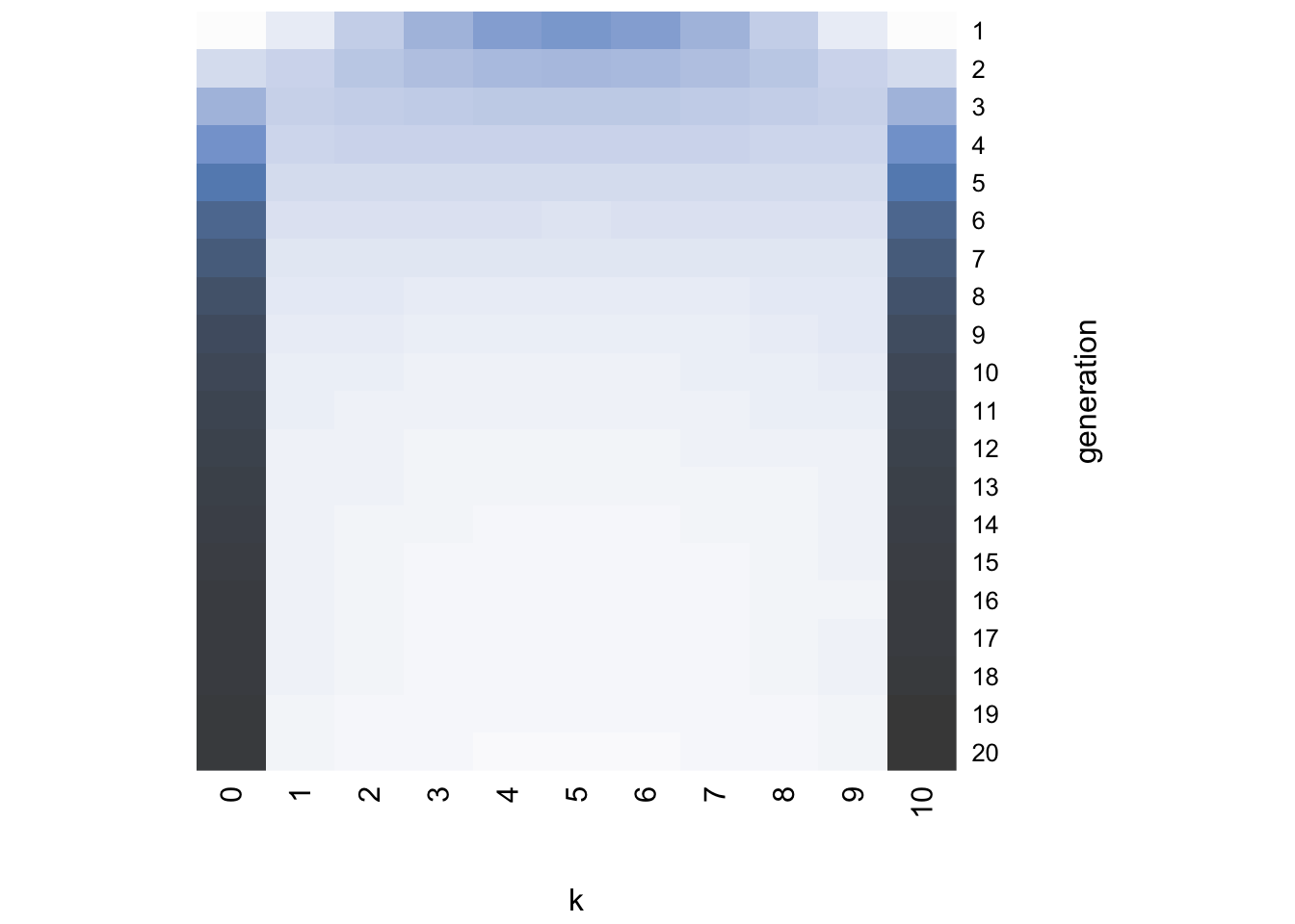
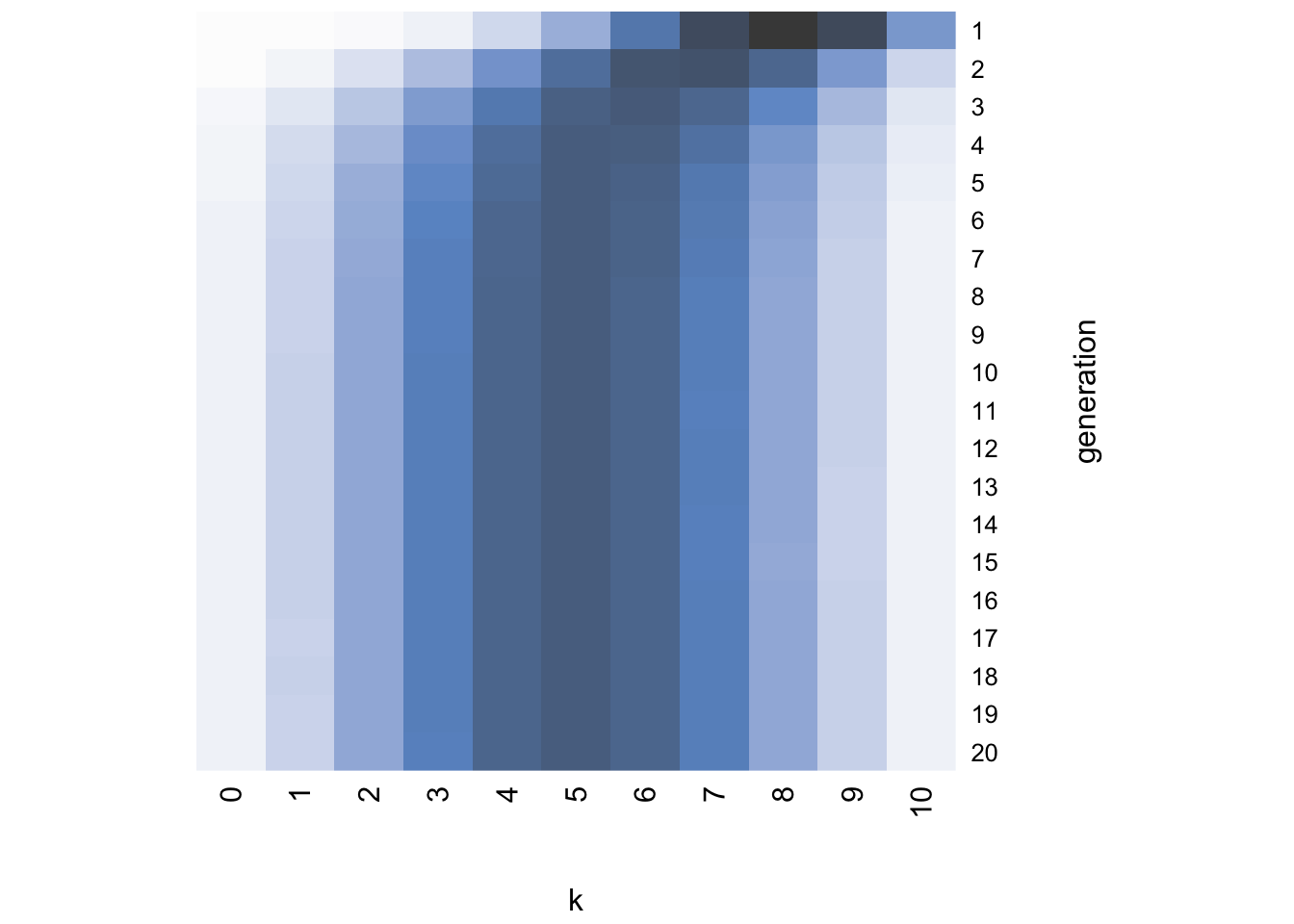
}I’ll leave you to play around with the different arguments of heatmap and read its help function, but essentially the command above creates a plot with generation on the vertical axis starting at the top, \(k\) on the horizontal axis, and the darkness of each cell indicating the probability of that \(k\) value in that generation. Darker colors indicate higher probabilities. For example, with the default \(\alpha = 1\), a flat prior, we generate this heatmap:
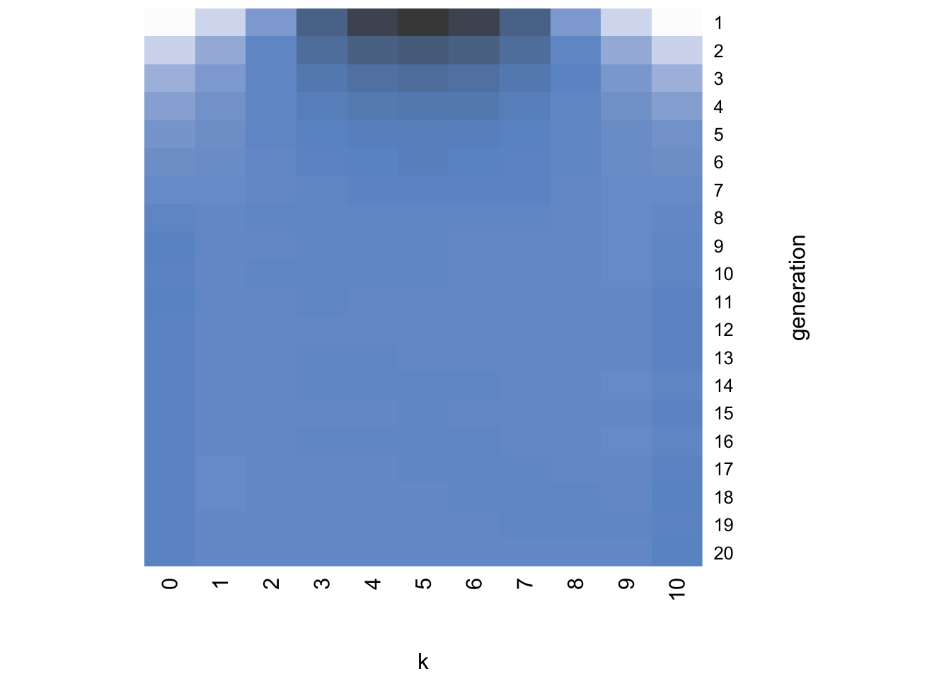
While generation 1 at the top resembles the likelihood concentrated around \(k = 5\), in just a few generations the distribution becomes uniform with roughly equal probability of each value of \(k\). In other words, the distribution has converged on the flat prior.
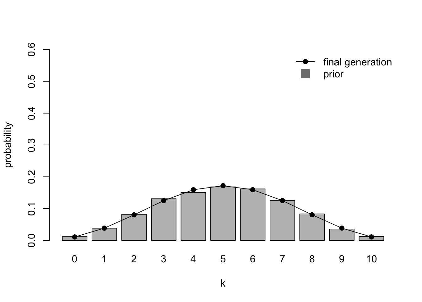
To compare the final generation more precisely with the priors, we can generate a plot from Navarro et al. (2018, Fig 3). Here we simulate \(r_{max}\) draws of \(\theta\) direct from the prior distribution, without any likelihoods or posteriors. We use this \(\theta\) to generate a \(k\) value like we did before, then calculate the proportion of each \(k\) value from 0 to \(n\). This is plotted as a bar plot using the barplot command, along with the final generation iterated learning probability distribution as a line.
IteratedFinalPlot <- function(data_model16, ymax = 0.6) {

  # retrieve parameters
  n <- data_model16$parameters["n"]
  r_max <- data_model16$parameters["r_max"]
  alpha <- data_model16$parameters["alpha"]
  beta <- data_model16$parameters["beta"]
  k_matrix <- data_model16$k_matrix

  # simulate prior distribution
  prior_dist <- rep(NA, r_max)

  for (i in 1:r_max) {

      theta <- rbeta(1, alpha, beta)
      prior_dist[i] <- rbinom(1, n, theta)

  }

  prior_dist <- table(factor(prior_dist, levels = 0:n))
  prior_dist <- prior_dist / sum(prior_dist)

  # draw barplot for simulated priors
  b <- barplot(height = prior_dist,
               names = 0:(length(prior_dist)-1),
               xlab = "k",
               ylab = "probability",
               ylim = c(0,ymax))

  # add line for the final generation iterated learning chain
  lines(k_matrix[nrow(k_matrix),],
        x = b,
        pch = 19,
        type = 'o')

  # add legend
  legend("topright",
         legend=c("final generation","prior"),
         pch = c(19,15),
         col=c("black","grey50"),
         pt.cex=c(1,2),
         bty="n",
         lty=c(1,NA),
         lwd=c(1,1))

}

IteratedFinalPlot(data_model16)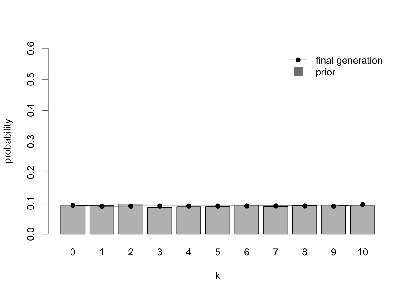
Here we confirm that after \(N = 20\) generations the initial data (\(k = 5\)) is overridden by the flat prior.
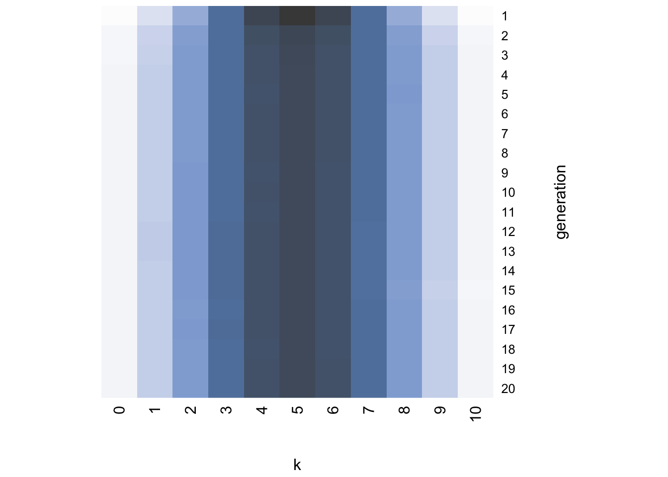
Now we create plots for a regularisation prior:
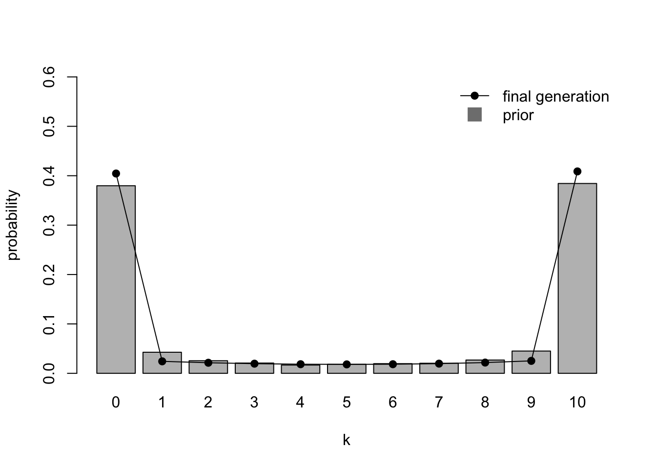
Strikingly, the heatmap shows that even though the first few generations retain the normal distribution of the likelihood, the chains soon converge on either \(k = 0\) or \(k = 10\). The final distribution plot confirms that the chains have converged on the prior.
And finally for an irregularisation prior:
Again, the final generation converges on the irregularisation prior, favouring languages that have a mix of the two grammatical variants.
We can now state our interim conclusion: despite all of the posteriors looking roughly the same after one generation, resembling a normal distribution centred around \(k / n = 0.5\), after 20 generations the population has converged on the prior distribution in each case. This is the conclusion reached by Reali & Griffiths (2009) and several other Bayesian iterated learning models and experiments. Try different values of \(k\) to confirm that this convergence on the priors is robust to any starting data. For example, a starting \(k = 10\) with irregularising priors (\(\alpha = 5\)) converges on those normally-distributed priors fairly rapidly:
While this is an important result, there are cases when iterated learning chains do not converge on the prior. One such case was explored by Navarro et al. (2018). So far we have assumed that all agents have identical priors. However, in many real world situations it is unlikely that everyone has the same priors. People come to problems with different expectations and past experiences, while some people may be more confident or certain than others.
Navarro et al. (2018) therefore assumed two different prior distributions, i.e. two sets of prior parameters. Each agent in the iterated learning chain uses parameters \(\alpha_1\) and \(\beta_1\) with probability \(h\), and uses \(\alpha_2\) and \(\beta_2\) with probability \(1 - h\).
The following function MixedIteratedLearning modifies IteratedLearning to accept two sets of prior parameters. With probability \(h\) the first set is passed to BayesianInference, and with probability \(1 - h\) the second set is passed. Otherwise everything is the same. Note the default parameter values are set so that if only \(\alpha_1\) and \(\beta_1\) are set, these values are copied to \(\alpha_2\) and \(\beta_2\).
MixedIteratedLearning <- function(n = 10,
                                  k = 5,
                                  alpha1 = 1,
                                  beta1 = alpha1,
                                  alpha2 = alpha1,
                                  beta2 = beta1,
                                  h = 0.5,
                                  sampling = TRUE,
                                  N = 20,
                                  r_max = 10000) {

  # vector to hold N k values
  k_vector <- rep(0, N)

  # matrix to hold N probability distributions for k
  k_matrix <- matrix(0, nrow = N, ncol = n+1)

  # record starting k
  k_initial <- k

  for (r in 1:r_max) {

    # reset k
    k <- k_initial

    # N probabilities that learner uses alpha1/beta1 rather than alpha2/beta2
    h_prob <- runif(N)

    for (i in 1:N) {

      if (h_prob[i] < h) {

        # alpha1 and beta1
        next_gen <- BayesianInference(n,
                                      k,
                                      alpha = alpha1,
                                      beta = beta1,
                                      sampling)

      } else {

        # alpha2 and beta2
        next_gen <- BayesianInference(n,
                                      k,
                                      alpha = alpha2,
                                      beta = beta2,
                                      sampling)

      }

      # k for next generation
      k <- next_gen$k

      # store probability distribution and k
      k_vector[i] <- k_vector[i] + next_gen$k
      k_matrix[i,] <- k_matrix[i,] + next_gen$prob_k

    }

  }

  # average across all runs
  k_vector <- k_vector / r_max
  k_matrix <- k_matrix / r_max

  # export k_vector, k_matrix and parameters
  list(k_vector = k_vector,
       k_matrix = k_matrix,
       parameters = c(n = n,
                      k = k_initial,
                      alpha1 = alpha1,
                      beta1 = beta1,
                      alpha2 = alpha2,
                      beta2 = beta2,
                      h = h,
                      sampling = sampling,
                      N = N,
                      r_max = r_max))

}
We also update IteratedFinalPlot to calculate the prior bars using the additional set of prior parameters:
IteratedFinalPlot <- function(data_model16, ymax = 0.6) {

  # retrieve parameters
  n <- data_model16$parameters["n"]
  r_max <- data_model16$parameters["r_max"]
  alpha1 <- data_model16$parameters["alpha1"]
  beta1 <- data_model16$parameters["beta1"]
  alpha2 <- data_model16$parameters["alpha2"]
  beta2 <- data_model16$parameters["beta2"]
  h <- data_model16$parameters["h"]
  k_matrix <- data_model16$k_matrix

  # simulate prior distribution
  prior_dist <- rep(NA, r_max)
  h_prob <- runif(r_max)

  for (i in 1:r_max) {

    if (h_prob[i] < h) {

      theta <- rbeta(1, alpha1, beta1)
      prior_dist[i] <- rbinom(1, n, theta)

    } else {

      theta <- rbeta(1, alpha2, beta2)
      prior_dist[i] <- rbinom(1, n, theta)

    }

  }

  prior_dist <- table(factor(prior_dist, levels = 0:n))
  prior_dist <- prior_dist / sum(prior_dist)

  # draw barplot for simulated priors
  b <- barplot(height = prior_dist,
               names = 0:(length(prior_dist)-1),
               xlab = "k",
               ylab = "probability",
               ylim = c(0,ymax))

  # add line for the final generation iterated learning chain
  lines(k_matrix[nrow(k_matrix),],
        x = b,
        pch = 19,
        type = 'o')

  # add legend
  legend("topright",
         legend=c("final generation","prior"),
         pch = c(19,15),
         col=c("black","grey50"),
         pt.cex=c(1,2),
         bty="n",
         lty=c(1,NA),
         lwd=c(1,1))

}
Navarro et al. (2018) wanted to simulate a population of agents with priors that favour different values of \(k\) and priors that differ in strength. Specifically, where some agents have weak priors for large values of \(k\) (\(\alpha_1 = 2, \beta_1 = 1\)), and some agents have strong priors for small values of \(k\) (\(\alpha_2 = 1, \beta_2 = 10\)). First let’s visualise these two sets of priors in homogenous populations, before simulating a heterogenous population. The following code first runs a simulation where all agents have weak priors for large values of \(k\), then a simulation where all agents have strong priors for small values of \(k\), plotting each side-by-side.
par(mfrow=c(1,2))

IteratedFinalPlot(MixedIteratedLearning(alpha1 = 2,
                                        beta1 = 1))

IteratedFinalPlot(MixedIteratedLearning(alpha1 = 1,
                                        beta1 = 10))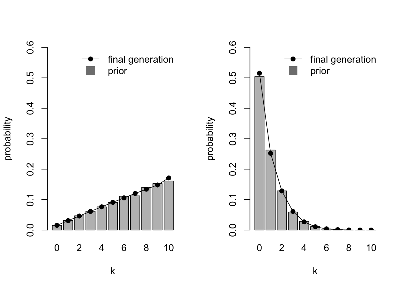
You can see how the left-hand prior distribution favours \(k = 10\) and the right-hand prior distribution favours \(k = 0\), and that the latter represents much more certainty in \(k = 0\) (about \(p = 0.5\)) than the former has in \(k = 10\) (about \(p = 0.175\)). As before, the final generation distributions almost exactly match the priors.
Now we run a mixed population where half (\(h = 0.5\), the default) of the agents have weak priors and half have strong priors:
par(mfrow=c(1,1))

IteratedFinalPlot(MixedIteratedLearning(alpha1 = 2,
                                        beta1 = 1,
                                        alpha2 = 1,
                                        beta2 = 10))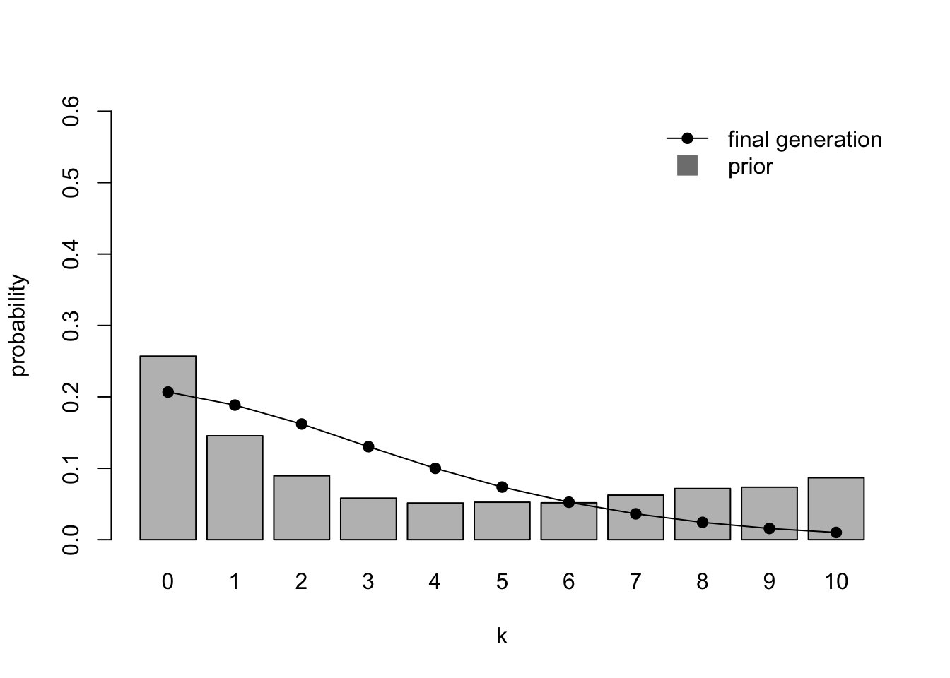
Here we have recreated Navarro et al.’s (2018) Fig 3. Unlike homogenous populations, heterogenous populations do not converge on the average of the different priors (the grey bars). They also don’t converge on either of the two prior distributions of the agents (shown in the previous two plots). Extreme values (\(k = 0\) and \(k > 6\)) are under-represented, while low non-zero values are over-represented. This is because the (1,10) priors favouring low values are stronger than the weak (2,1) priors favouring high values. The greater certainty of the former exerts a disproportionate influence on the iterated learning chain.
Another case where iterated learning chains do not converge exactly on the priors is when MAP is used instead of sampling. Recall that MAP selects the value of \(\theta\) with the maximum posterior probability, while sampling picks \(\theta\) randomly in proportion to the posterior. This can be seen with the weak and strong homogenous priors we just simulated, changing sampling to FALSE.
par(mfrow=c(1,2))

IteratedFinalPlot(MixedIteratedLearning(alpha1 = 2,
                                        beta1 = 1,
                                        sampling = FALSE))

IteratedFinalPlot(MixedIteratedLearning(alpha1 = 1,
                                        beta1 = 10,
                                        sampling = FALSE),
                  ymax = 0.8)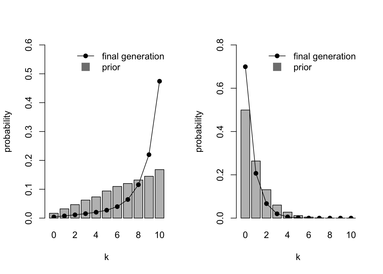
MAP exaggerates the prior distribution. For the weak priors favouring large values of \(k\) (the left hand plot), \(k = 9\) and \(k = 10\) are greatly over-represented in the final generation compared to the relatively smooth priors. For the strong priors favouring small values of \(k\) (the right hand plot), \(k = 0\) is over-represented. This tendency for MAP to exaggerate the prior distribution has been reported in previous models (e.g. Kirby et al. 2007).
Finally, we can combine the previous two cases to simulate a mixed population of MAP agents where the vast majority (95%, i.e. \(h = 0.95\)) are unbiased with flat priors (\(\alpha_1 = \beta_1 = 1\)), and a small minority (5%) are extremely biased towards one of the variants (\(\alpha_2 = 1, \beta_2 = 100\)):
IteratedFinalPlot(MixedIteratedLearning(alpha1 = 1,
                                        beta1 = 1,
                                        alpha2 = 1,
                                        beta2 = 100,
                                        h = 0.95,
                                        sampling = FALSE))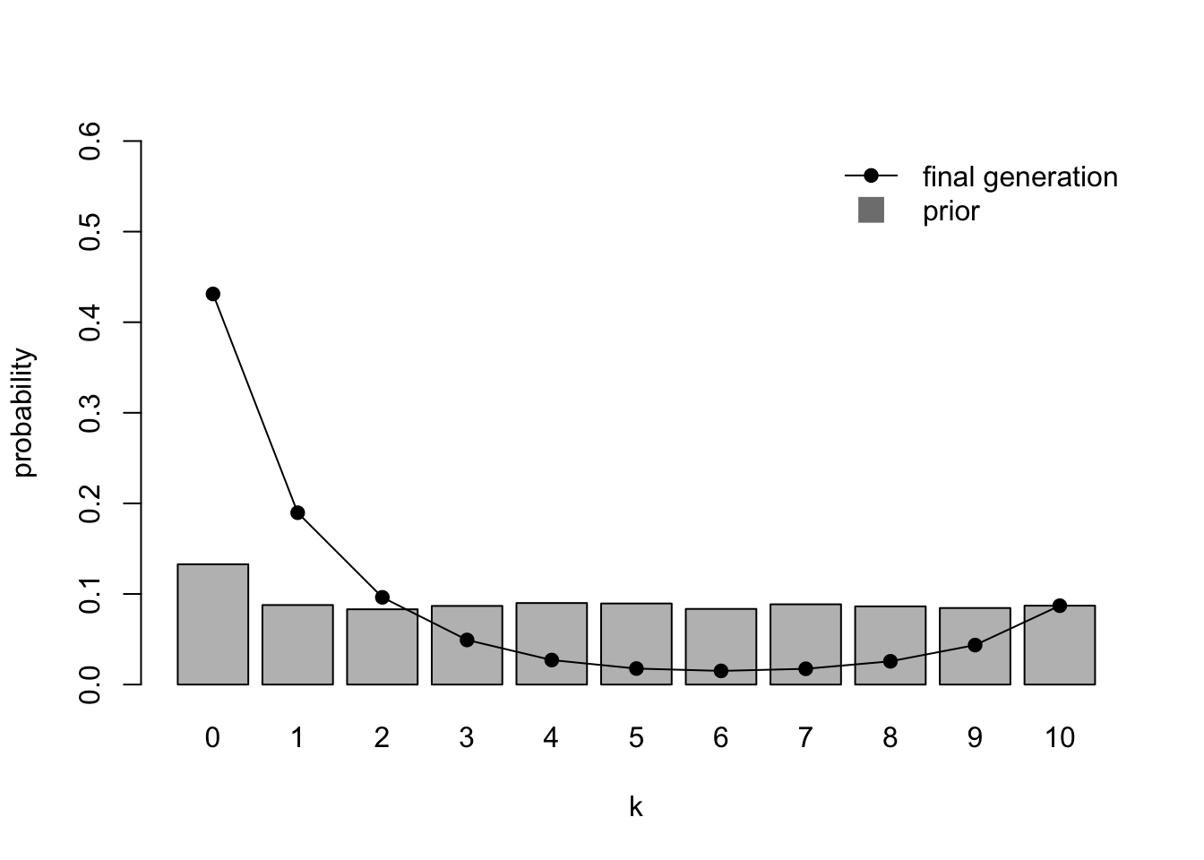
Here the final generation distribution looks very different to the almost flat priors. The small minority who have extreme beliefs in one variant skew the unbiased majority towards that variant.
Summary
Model 16 combined Bayesian inference with iterated learning to explore the cultural evolution of linguistic regularisation. Bayesian inference provides a way of integrating the likelihood of some data with prior expectations to generate a posterior probability distribution over all possible hypotheses. Iterated learning places Bayesian learners in a chain, with each learner producing data for the next participant from their posterior distribution. While this was discussed in terms of regularisation in language, this general approach has been used to study the cultural evolution of a range of linguistic and cognitive features and offers an alternative to the population-genetics-inspired models of previous chapters.
The key result of Model 16 is that chains typically converge on individuals’ priors irrespective of the starting data, as concluded by Reali & Griffiths (2009). This is not obvious from a single learning episode, and only occurs after several generations of repeated learning and cultural transmission. This suggests that if in the real world we see languages that are mostly regular, then people possess priors that reflect this. In the model, this would be an \(\alpha\) less than one. Indeed, Reali & Griffiths (2009) ran an iterated learning experiment resembling this model and found that participants’ choices were consistent with them having \(\alpha = 0.052\), a strong regularisation prior. In a similar experiment, Ferdinand et al. (2013) found \(\alpha = 0.605\), not as extreme but still less than one, so again indicating a regularisation bias.
Where do these priors come from? It is possible that they are innate (i.e. genetically specified), supporting nativist approaches to language evolution commonly identified with Noam Chomsky. However, this is not necessarily the case: priors could also be the result of how human cognition or learning works in general, without being specific to language. One might imagine that regular grammatical rules are easier to learn and remember than irregular forms. Priors might also be themselves culturally acquired, which can be captured by hierarchical Bayesian models (Kemp et al. 2007).
This Bayesian iterated learning approach has been more generally applied than just regularisation (e.g. to compositionality: Kirby et al. 2007; Smith & Kirby 2008), and just language. Any culturally transmitted cognitive representation can be modelled in this way, from object categorisation to color terminologies (e.g. Griffiths et al. 2008). Can we apply Reali & Griffiths’ (2009) conclusion that cultural forms always reflect individual priors to all of human culture? This is certainly consistent with ‘cultural attraction’ approaches to cultural evolution (Claidière & Sperber 2007), which holds that stable patterns of cultural variation can be explained in terms of individual-level cognitive biases.
However, we should remember that there were two cases where cultural evolution did not converge on the priors in Model 16. When agents had different priors, iterated learning did not converge on any single agent’s priors, nor on the average of all agents’ priors (Navarro et al. 2018). In the final case we considered, a small minority with extreme priors disproportionately influenced cultural dynamics when the rest of the population had flat priors. Such a case does not seem unrealistic in an age when a small number of people with extreme opinions are highly visible on social media and may disproportionately influence the silent majority.
The second case was when agents chose the ‘maximum a posteriori’ (MAP) hypothesis from the posterior rather than sampled randomly from the posterior. Iterated learning with MAP exaggerates the prior distribution. This result has been used to argue that the distinctive patterns of cultural variation we see in the real world can be generated by very weak biases at the individual level, given that MAP magnifies these biases (Kirby et al. 2007). Do real people use sampling or MAP? The evidence is mixed. Reali & Griffiths (2009) found that their participants better resembled samplers, and Bonawitz et al. (2014) summarise evidence for sampling in children, whereas Smith & Kirby (2008) show that MAP is more evolutionarily stable than sampling.
We should also remember that there is no selection or cultural accumulation in these models. In real life, cognitively intuitive ideas and practices such as miasma theory or creationism have been replaced with more accurate but less intuitive concepts such as germ theory or evolutionary theory. While language may be a special case, there are likely many other realms of cultural evolution where cultural forms do not resemble people’s priors due to cultural selection (see Mesoudi 2021).
Model 16 introduced a few new tools to our modelling toolkit. We made heavy use of statistical distributions (the binomial and the beta), we saw how to implement Bayes’ rule, and how to use conjugate priors to speed up code. We used the heatmap function to visualise the data probability distribution over time, and barplot to plot the priors. Finally, unlike previous simulation functions which incorporated plotting code, we created two separate plot functions that took the function output as input. A handy trick is to include the simulation function parameters in the output, when they are needed by the plotting functions.
Acknowledgements
For this model I am grateful to Simon Kirby for sharing his Masters course code, and Danielle Navarro for releasing the R code for Navarro et al. (2018) upon which Model 16 is based.
Exercises
Create a function that, for given values of \(n\), \(k\) and \(\alpha\), uses BayesianInference to generate three plots one above the other, one showing the likelihood, one showing the prior, and one showing the posterior. Try different values of \(n\), \(k\) and \(\alpha\) to explore how priors and likelihoods combine to generate posterior distributions.
Try different values of \(\alpha\) in IteratedLearning to confirm that \(\alpha < 1\) generates regularisation and \(\alpha > 1\) generates irregularisation. Also try setting \(\beta\) to different values than \(\alpha\) to see whether iterated learning chains converge on asymmetrical priors.
Simulate a population that is highly polarised in their prior opinions, with 50% possessing \(\alpha_1 = 1, \beta_1 = 100\) priors and 50% possessing \(\alpha_2 = 100, \beta_2 = 1\) priors. Do the chains reach a consensus or do they remain as polarised as the priors? Does this differ from the patterns observed in Model 10 (Polarisation)? If so, why?
Rather than \(h\) being the probability of a single agent using the first set of priors, make \(h\) the probability of an entire chain using the first set of priors. How does this change the cultural dynamics of the iterated learning chains?
Another extension that potentially prevents convergence on the prior is having multiple individuals in each generation of the iterated learning chain (Ferdinand & Zuidema 2009). Create a new simulation function MultiAgentIteratedLearning which contains \(g\) agents per generation. Each agent generates \(n\) utterances, and the subsequent \(g\) agents in the next generation use all \(gn\) utterances as their input. Do chains with \(g > 1\) recapitulate the priors?
References
Bonawitz, E., Denison, S., Griffiths, T. L., & Gopnik, A. (2014). Probabilistic models, learning algorithms, and response variability: sampling in cognitive development. Trends in cognitive sciences, 18(10), 497-500.
Claidière, N., & Sperber, D. (2007). The role of attraction in cultural evolution. Journal of Cognition and Culture, 7(1-2), 89-111.
Ferdinand, V., & Zuidema, W. (2009). Thomas’ theorem meets Bayes’ rule: A model of the iterated learning of language. In Proceedings of the Annual Meeting of the Cognitive Science Society (Vol. 31, No. 31).
Ferdinand, V., Kirby, S., & Smith, K. (2014). Regularization in language evolution: On the joint contribution of domain-specific biases and domain-general frequency learning. In Evolution of Language: Proceedings of the 10th International Conference (EVOLANG10) (pp. 435-436).
Griffiths, T. L., Christian, B. R., & Kalish, M. L. (2008). Using category structures to test iterated learning as a method for identifying inductive biases. Cognitive Science, 32(1), 68-107.
Kemp, C., Perfors, A. & Tenenbaum, J. B. (2007). Learning overhypotheses with hierarchical Bayesian models. Developmental Science, 10, 307–321.
Kirby, S., Dowman, M., & Griffiths, T. L. (2007). Innateness and culture in the evolution of language. Proceedings of the National Academy of Sciences, 104(12), 5241-5245.
Mesoudi, A. (2021). Cultural selection and biased transformation: two dynamics of cultural evolution. Philosophical Transactions of the Royal Society B, 376(1828), 20200053.
Navarro, D. J., Perfors, A., Kary, A., Brown, S. D., & Donkin, C. (2018). When extremists win: Cultural transmission via iterated learning when populations are heterogeneous. Cognitive Science, 42(7), 2108-2149.
Perfors, A., Tenenbaum, J. B., Griffiths, T. L., & Xu, F. (2011). A tutorial introduction to Bayesian models of cognitive development. Cognition, 120(3), 302-321.
Reali, F., & Griffiths, T. L. (2009). The evolution of frequency distributions: Relating regularization to inductive biases through iterated learning. Cognition, 111(3), 317-328.
Smith, K., & Kirby, S. (2008). Cultural evolution: implications for understanding the human language faculty and its evolution. Philosophical Transactions of the Royal Society B, 363(1509), 3591-3603.