Model 10: Polarization
Introduction
A central question in cultural evolution research is how cultural diversity is generated and maintained. One counter-intuitive answer to this question was offered by Axelrod (1997) using what has become an influential agent-based model. Axelrod showed that regional differences in cultural traits - or ‘polarization’ when neighbouring regions are maximally culturally different to one another - can be generated and maintained even though individual agents are trying to become as similar as possible to other agents. In Axelrod’s terminology, global cultural divergence at the population level can emerge despite local cultural convergence at the individual level. This conclusion has implications for a variety of social phenomena, from political polarization in social media to racial segregation in cities.
Axelrod demonstrated this using a spatially explicit agent-based model. ‘Spatially explicit’ means that rather than a homogenous mass of agents existing all with an equal probability of interacting with any other agent, instead each agent exists in a specific location in space, with a set of neighbouring agents with whom they may be more likely to interact than agents further away in space. Agent-based models are particularly suited for this kind of spatially explicit simulation compared to analytical models. Our previous models have already incorporated non-random interaction between agents and minimal population structure, such as the assortative cultural mating of Model 6 (vertical/horizontal transmission) and the movement across groups of Model 7 (migration). In Model 10 we will go further and recreate Axelrod’s classic model, learning how to create and analyse spatially explicit agent-based models where each agent inhabits a specific position in a spatial grid.
Another distinct feature of Axelrod’s model is his assumption that agents possess multiple cultural traits, and these can serve as markers of identity and influence interaction. Specifically, he assumed that each agent possesses a number of cultural ‘features’. Each feature can take on one of several trait values. In his basic model, there are five cultural features, each of which can take one of ten possible trait values. When modelling cultural diversity, it makes sense to model multiple cultural traits. Each member of a real society possesses multiple culturally-transmitted traits - language(s) spoken, dialects of those languages, dress customs, whether cars are driven on the left or the right, using knives and forks or chopsticks, bowing vs handshakes, etc. These traits in combination - rather than any single trait - define a society’s culture. While we modelled two cultural traits in Model 4 (indirect bias), in Model 10 we will model more than two.
Axelrod’s model, like all good agent-based models, is simple. Each agent is placed in a fixed position on a square grid. There are \(N_{side}\) agents along each side of the grid, giving \({N_{side}}^2\) agents in total. Each agent has \(g = 5\) cultural features. Each feature takes one of ten values, denoted with the integers 0-9. For example, an agent might have traits 58290. Here, the first feature is 5, the second 8, and so on.
In the first timestep each agent’s trait values are picked at random. Then in each timestep, the following three rules are applied:
Pick an agent at random (the focal agent)
Pick one of the focal agent’s neighbours at random. A neighbour is an agent to the immediate north, south, east or west of the focal agent’s grid position. Focal agents at the corner or edge of the grid may have no neighbour in one of those positions, and so have only two or three neighbours respectively.
With probability equal to the proportion of shared cultural traits between the focal agent and its chosen neighbour, pick one feature at random that differs between focal agent and its neighbour, and set the focal agent’s value of that feature to the neighbour’s value.
These rules plausibly assume that agents are more likely to interact with, and be influenced by, other agents to the extent that they are culturally similar, as indexed by the proportion of cultural traits that they share. When two agents are completely dissimilar, then the proportion of shared features will be zero, and no interaction / influence will occur. The more traits they share, the more likely they are to interact and potentially become even more similar.
The outcome that we are interested in is the cultural diversity or homogeneity that emerges after a certain number of timesteps, or iterations of the above three rules. The only cultural change that can occur according to the three rules above is that agents become more similar to one another. There is no mutation, and no rules that make agents more dissimilar. We would expect, therefore, that all agents will gradually become more and more similar, perhaps identical, and eventually every agent will be culturally identical.
Model 10
Let’s build the model step by step before putting it together in a function. First we need to create agents and their traits. Rather than a dataframe, we will use a matrix. A matrix is perfect because it has a fixed number of rows and columns, and these rows and columns will serve as the coordinates for our spatial grid. In our case the matrix will be square, with \(N_{side}\) rows and \(N_{side}\) columns. Each agent inhabits a fixed position in the matrix. Indexing starts at the top left and has the notation [row,column]. The agent in the top left position is therefore at position [1,1]; its neighbour to the east is in position [1,2]; and its neighbour to the south is at [2,1].
First we create a 10x10 matrix (i.e. \(N_{side} = 10\)) filled for now with NAs:
N_side <- 10

# make agent matrix of size N_size x N_size
agent <- matrix(NA,
                nrow = N_side,
                ncol = N_side)

agent
## [,1] [,2] [,3] [,4] [,5] [,6] [,7] [,8] [,9] [,10]
## [1,] NA NA NA NA NA NA NA NA NA NA
## [2,] NA NA NA NA NA NA NA NA NA NA
## [3,] NA NA NA NA NA NA NA NA NA NA
## [4,] NA NA NA NA NA NA NA NA NA NA
## [5,] NA NA NA NA NA NA NA NA NA NA
## [6,] NA NA NA NA NA NA NA NA NA NA
## [7,] NA NA NA NA NA NA NA NA NA NA
## [8,] NA NA NA NA NA NA NA NA NA NA
## [9,] NA NA NA NA NA NA NA NA NA NA
## [10,] NA NA NA NA NA NA NA NA NA NAThe rows are labelled along the left hand side, and the columns along the top.
Now we need \(g\) features each of which initially takes one integer from 0 to 9. The following code sets \(g = 5\), and then uses sample.int to pick \(g\) integers from 0 to 9, with replacement (so integers can repeat). Note that the sample.int command returns random integers from one up to the first argument. Because we want to include 0 as a trait, we pick random integers from 1 to 10, then subtract 1 to get the range 0 to 9.
## [1] 3 2 1 0 2Because we want each one to fit into a single cell of the matrix, we need to condense them into a single value. We could turn them into a \(g\)-digit number. However, this would lose the leading zeroes (e.g. 0 0 4 8 5 would become 485, not 00485). Instead we will convert to a character (chr) variable, using the paste command with collapse = “” to remove the spaces:
## [1] "01801"Now we can fill the agent matrix with random traits and display them (the options command simply widens the print area on the pdf output to see the matrix properly).
  # fill agent with g numbers each a random integer 0-9, stored as chr
  for (n_width in 1:N_side) {

    for (n_height in 1:N_side) {

      agent[n_width,n_height] <- paste(sample.int(10, g, replace = TRUE) - 1,
                                       collapse = "")

    }

  }

options(width = 300)
agent
## [,1] [,2] [,3] [,4] [,5] [,6] [,7] [,8] [,9] [,10]
## [1,] "54574" "58439" "47909" "89826" "23499" "10235" "88027" "80522" "02924" "28904"
## [2,] "71211" "37108" "61655" "10090" "71306" "45511" "09503" "90431" "96903" "93772"
## [3,] "59153" "88574" "90577" "93976" "88398" "36334" "71312" "12911" "26261" "78674"
## [4,] "38495" "28572" "36800" "22024" "16342" "86360" "20187" "91382" "07069" "99701"
## [5,] "49697" "46517" "71600" "98616" "64313" "45351" "18232" "21924" "54064" "34946"
## [6,] "33368" "70276" "79404" "45280" "32314" "21421" "64626" "46646" "62840" "85417"
## [7,] "20042" "30591" "31661" "57422" "02216" "32355" "11301" "14146" "40871" "18512"
## [8,] "20879" "35327" "10877" "06711" "98806" "73134" "77053" "91808" "38313" "66392"
## [9,] "40246" "16482" "92934" "02339" "33820" "41454" "46741" "16288" "86557" "68516"
## [10,] "09651" "93996" "08398" "09656" "60874" "10433" "71411" "96043" "12394" "35120"Here we have reproduced Table 1 from Axelrod (1997): a 10 x 10 grid containing \(g\)-length cultural traits for 100 agents.
Now to convert the three rules above into code. First we pick a random agent to be the focal agent. We do this by picking a random row value and a random column value, and setting focal to the agent in that position.
# pick a focal agent at random
focal_row <- sample(1:N_side, 1)
focal_col <- sample(1:N_side, 1)
focal <- agent[focal_row, focal_col]

focal
## [1] "34946"Now we pick one of the focal’s neighbours at random, as per rule 2. This is complicated by the fact that some focal agents will have four neighbours (those in the middle of the grid), some will have three (those at the edges) and some will have only two (those in the corners). We don’t want to pick a non-existent neighbour to compare with the focal. The following code creates a vector of all_neighbours, adds (‘appends’) to this vector only those neighbours that exist given the focal’s position, and picks one of the existing neighbours at random to be the neighbour.
# pick one of its neighbours at random
# ignoring non-existent agents outside boundaries

all_neighbours <- NULL

if (focal_row-1 >= 1)
  all_neighbours <- append(all_neighbours,
                           agent[focal_row-1, focal_col])
if (focal_row+1 <= N_side)
  all_neighbours <- append(all_neighbours,
                           agent[focal_row+1, focal_col])
if (focal_col-1 >= 1)
  all_neighbours <- append(all_neighbours,
                           agent[focal_row, focal_col-1])
if (focal_col+1 <= N_side)
  all_neighbours <- append(all_neighbours,
                           agent[focal_row, focal_col+1])

neighbour <- sample(all_neighbours, 1)

neighbour
## [1] "54064"We can now simulate rule 3, the cultural change. First we convert the focal and neighbour’s traits from a single character into numbers using the unlist and strsplit commands. This is essentially the reverse of the paste command above. We can then get the cultural similarity between focal and neighbour by adding the number of features that are identical and dividing by the total number of features. Then, if this similarity is greater than zero and less than one, i.e. the two agents are not completely dissimilar nor identical, then with probability equal to similarity we pick a random feature that differs between the focal and neighbour and store it as feature. These are identified using the which command (i.e. which(focal != neighbour)). If there is a single dissimilar feature (i.e. sum(focal != neighbour) == 1) then this single dissimilar feature is stored in feature. If there is more than one, then we pick one at random using sample. Note that we do this because, if there is a single dissimilar feature, sample will not work properly. Always make sure sample is picking from more than one numeric element, never a single numeric element (try running sample(2, 10, replace = TRUE) to see this). Finally, we set the focal agent’s chosen dissimilar trait value to that of its neighbour, and insert the modified focal traits back into the agent matrix.
# separate out traits and make them numeric, for comparing
focal <- as.numeric(unlist(strsplit(focal, split = NULL)))
neighbour <- as.numeric(unlist(strsplit(neighbour, split = NULL)))

# get similarity
similarity <- sum(focal == neighbour) / length(focal)

if (similarity > 0 & similarity < 1) {

  if (runif(1) < similarity) {

    if (sum(focal != neighbour) == 1) {
      feature <- which(focal != neighbour)
    } else {
      feature <- sample(which(focal != neighbour), 1)
    }

    focal[feature] <- neighbour[feature]

    agent[focal_row, focal_col] <- paste(focal, collapse = "")

  }

}

paste(focal, collapse = "")
## [1] "34946"## [1] "54064"## [1] 0.2## [1] "34946"The output shows the original focal agent, its neighbour, their similarity, and the modified focal agent. The latter may well be identical to the original focal traits, given that our randomised agents are currently highly dissimilar to one another (probably similarity = 0, in which case there is definitely no change). Try repeating the above code but with the focal and neighbour set to be maximally similar without being identical, e.g. “12345” and “12340” respectively. In this case similarity = 0.8 and the final feature in focal is likely to flip from 5 to 0.
We now have all the code to write a function. Polarization below combines all the previous code, wrapping the three rules in a loop to repeat them \(t_{max}\) times. The output of the simulation is the final agent matrix at \(t = t_{max}\) and the number of timesteps at which this was produced (this will be used later when plotting the results).
Polarization <- function(N_side, g, t_max) {

  # make agent matrix of size N_size x N_size
  agent <- matrix(NA,
                  nrow = N_side,
                  ncol = N_side)

  # fill agent with g numbers each a random integer 0-9, stored as chr
  for (n_width in 1:N_side) {

    for (n_height in 1:N_side) {

      agent[n_width,n_height] <- paste(sample.int(10, g, replace = TRUE) - 1,
                                       collapse = "")

    }

  }

  for (t in 1:t_max) {

    # pick a focal agent at random
    focal_row <- sample(1:N_side, 1)
    focal_col <- sample(1:N_side, 1)
    focal <- agent[focal_row, focal_col]

    # pick one of its neighbours at random
    # ignoring non-existent agents outside boundaries

    all_neighbours <- NULL

    if (focal_row-1 >= 1)
      all_neighbours <- append(all_neighbours,
                               agent[focal_row-1, focal_col])
    if (focal_row+1 <= N_side)
      all_neighbours <- append(all_neighbours,
                               agent[focal_row+1, focal_col])
    if (focal_col-1 >= 1)
      all_neighbours <- append(all_neighbours,
                               agent[focal_row, focal_col-1])
    if (focal_col+1 <= N_side)
      all_neighbours <- append(all_neighbours,
                               agent[focal_row, focal_col+1])

    neighbour <- sample(all_neighbours, 1)

    # compare focal and neighbour agents:
    # if there's at least one dissimilar trait,
    # and with prob equal to the similarity between focal and neighbout,
    # set a random dissimilar focal trait to that of the neighbour's

    # separate out traits and make them numeric, for comparing
    focal <- as.numeric(unlist(strsplit(focal, split = NULL)))
    neighbour <- as.numeric(unlist(strsplit(neighbour, split = NULL)))

    # get similarity
    similarity <- sum(focal == neighbour) / length(focal)

    if (similarity > 0 & similarity < 1) {

      if (runif(1) < similarity) {

          if (sum(focal != neighbour) == 1) {
            feature <- which(focal != neighbour)
          } else {
            feature <- sample(which(focal != neighbour), 1)
          }

        focal[feature] <- neighbour[feature]

        agent[focal_row, focal_col] <- paste(focal, collapse = "")

      }

    }

  }

  # output agent matrix and t_max
  list(agent = agent, t = t)

}
Here is one run of the Polarization function, with \(N_{side} = 10\), \(g = 5\) and \(t_{max} = 100000\). We display the final agent matrix that has been stored in data_model10.
##       [,1]    [,2]    [,3]    [,4]    [,5]    [,6]    [,7]    [,8]    [,9]    [,10]
##  [1,] "02696" "02696" "02696" "02696" "02696" "02696" "02696" "02696" "02696" "02696"
##  [2,] "02696" "02696" "02696" "02696" "02696" "02696" "02696" "02696" "02696" "02696"
##  [3,] "02696" "02696" "02696" "02696" "02696" "02696" "02696" "02696" "02696" "02696"
##  [4,] "02696" "02696" "02696" "02696" "02696" "02696" "02696" "02696" "02696" "02696"
##  [5,] "02696" "02696" "02696" "02696" "02696" "02696" "02696" "02696" "02696" "02696"
##  [6,] "02696" "02696" "02696" "02696" "02696" "02696" "02696" "02696" "02696" "02696"
##  [7,] "02696" "02696" "02696" "02696" "02696" "02696" "02696" "02696" "02696" "02696"
##  [8,] "02696" "02696" "02696" "02696" "02696" "02696" "02696" "02696" "02696" "86932"
##  [9,] "02696" "02696" "02696" "02696" "02696" "02696" "02696" "02696" "02696" "86932"
## [10,] "02696" "02696" "02696" "02696" "02696" "02696" "02696" "02696" "02696" "86932"
After 100,000 timesteps, there should be noticeable similarity in the agent traits above. Probably not complete similarity, however. While most agents should have the same traits, there should be some areas of the matrix where some agents have a different trait.
Axelrod plotted the output of the model using lines of different thickness to denote the cultural similarity between neighbouring agents. The function PolarizationPlot below does this, using the data_model10 output from Polarization. First we retrieve the agent matrix and \(t_{max}\) from data_model10, as well as \(N_{side}\) from agent. We then make an empty \(N_{side}\) x \(N_{side}\) plot, add a title recording the number of timesteps, and add lines around the sides using segments. Then we cycle through each agent along the rows (the Row loop) and columns (the Col loop) to draw vertical lines. We pick each agent and its neighbour to the east, calculate their similarity in the same way as we did above, set the lwd (line width) in proportion to the similarity, and draw a line using segments. Once all the vertical lines are drawn we cycle through again, this time comparing each agent to its neighbour to the south and drawing horizontal lines at the boundaries between them.
PolarizationPlot <- function(data_model10) {

  agent <- data_model10$agent
  t_max <- data_model10$t

  # retrieve N_side from matrix
  N_side <- dim(agent)[1]

  # make an empty N_side x N_side plot
  plot(NULL,
       ylim = c(0, N_side),
       xlim = c(0, N_side),
       ylab = "",
       xlab = "",
       axes = FALSE,
       main = paste("After ", format(t_max, scientific = F), " timesteps",
                    sep = ""))

  # add a frame around the edges
  segments(x0 = 0, y0 = 0,
           x1 = 0, y1 = N_side)
  segments(x0 = 0, y0 = 0,
           x1 = N_side, y1 = 0)
  segments(x0 = 0, y0 = N_side,
           x1 = N_side, y1 = N_side)
  segments(x0 = N_side, y0 = 0,
           x1 = N_side, y1 = N_side)

  # vertical lines

  for (Row in 1:N_side) {

    for (Col in 1:(N_side-1)) {

      # agent2 is to the right of agent1
      agent1 <- agent[Row,Col]
      agent2 <- agent[Row,Col+1]

      # make numeric
      agent1 <- as.numeric(unlist(strsplit(agent1, split = NULL)))
      agent2 <- as.numeric(unlist(strsplit(agent2, split = NULL)))

      # get similarity
      similarity <- sum(agent1 == agent2) / length(agent1)

      # set line thickness
      if (similarity < 1)    lwd <- 0.5
      if (similarity <= 0.8) lwd <- 1
      if (similarity <= 0.6) lwd <- 3
      if (similarity <= 0.4) lwd <- 5
      if (similarity <= 0.2) lwd <- 7

      if (similarity < 1) {

        segments(x0 = Col, x1 = Col,
                 y0 = N_side-Row, y1 = N_side-Row+1,
                 lwd = lwd)

      }

    }

  }

  # horizontal lines

  for (Row in 1:(N_side-1)) {

    for (Col in 1:N_side) {

      # agent2 is directly below agent1
      agent1 <- agent[Row,Col]
      agent2 <- agent[Row+1,Col]

      # make numeric
      agent1 <- as.numeric(unlist(strsplit(agent1, split = NULL)))
      agent2 <- as.numeric(unlist(strsplit(agent2, split = NULL)))

      # get similarity
      similarity <- sum(agent1 == agent2) / length(agent1)

      # set line thickness
      if (similarity < 1)    lwd <- 0.5
      if (similarity <= 0.8) lwd <- 1
      if (similarity <= 0.6) lwd <- 3
      if (similarity <= 0.4) lwd <- 5
      if (similarity <= 0.2) lwd <- 7

      if (similarity < 1) {

        segments(y0 = N_side-Row, y1 = N_side-Row,
                 x0 = Col-1, x1 = Col,
                 lwd = lwd)

      }

    }

  }

}
Below is the plot for the run created above. It should match the agent matrix, with lines separating agents that are dissimilar. The thicker the lines, the more dissimilar the agents are.
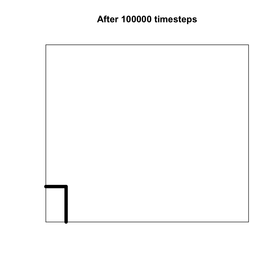
The plot should show a small number of regions that are dissimilar to the neighbouring regions. Despite individual agents’ preferences to interact with and copy similar others, different regions of the grid have polarized into groups with different cultural traits.
How many distinct regions are there in the plot above? We could count them visually, but better would be to use the code below. We convert the agent matrix to a vector, and count the number of unique traits using the unique command.
## [1] 2Note that this is the number of unique traits in the entire population. It may not be the same as the number of regions shown in the plot, if there are two non-contiguous regions that have the same trait. Axelrod doesn’t specify whether he recorded the number of unique traits or the number of non-contiguous regions. These are unlikely to differ too much though, as the chances of two non-contiguous regions having identical traits is slim.
How did these regions form over time? The function PolarizationMultiplot below creates a multi-panel 2 x 2 plot which plots the agent matrix at four different points of the same run, as in Axelrod’s Figure 1. The parameter \(t_{plot}\) replaces \(t_{max}\). \(t_{plot}\) is a list of four timesteps at which the output is plotted; the final value in \(t_{plot}\) will effectively therefore be \(t_{max}\). Most of the code in PolarizationMultiplot is the same as Polarization, except that we set up a 2 x 2 plot using par(mfrow = c(2,2)), store each of the four agent matrices in agent_list whenever the timestep \(t\) matches one of the \(t_{plot}\) values (using if (t %in% t_plot)), and plot each agent matrix using PolarizationPlot at the end.
PolarizationMultiplot <- function(N_side, g, t_plot) {

  # make agent matrix of size N_size x N_size
  agent <- matrix(NA,
                  nrow = N_side,
                  ncol = N_side)

  # fill agent with g-digit codes, stored as chr
  for (n_width in 1:N_side) {

    for (n_height in 1:N_side) {

      agent[n_width,n_height] <- paste(sample.int(10, g, replace = TRUE) - 1,
                                       collapse = "")

    }

  }

  # set up 2x2 plot panels
  par(mfrow = c(2,2))

  # set up agent list to store data
  agent_list <- list(NULL)

  for (t in 1:max(t_plot)) {

    # pick a focal agent at random
    focal_row <- sample(1:N_side, 1)
    focal_col <- sample(1:N_side, 1)
    focal <- agent[focal_row, focal_col]

    # pick one of its neighbours at random
    # ignoring non-existent agents outside boundaries

    all_neighbours <- NULL

    if (focal_row-1 >= 1)
      all_neighbours <- append(all_neighbours,
                               agent[focal_row-1, focal_col])
    if (focal_row+1 <= N_side)
      all_neighbours <- append(all_neighbours,
                               agent[focal_row+1, focal_col])
    if (focal_col-1 >= 1)
      all_neighbours <- append(all_neighbours,
                               agent[focal_row, focal_col-1])
    if (focal_col+1 <= N_side)
      all_neighbours <- append(all_neighbours,
                               agent[focal_row, focal_col+1])

    neighbour <- sample(all_neighbours, 1)

    # compare focal and neighbour agents:
    # if there's at least one dissimilar trait,
    # and with prob equal to the similarity between focal and neighbout,
    # set a random dissimilar focal trait to that of the neighbour's

    # separate out traits and make them numeric, for comparing
    focal <- as.numeric(unlist(strsplit(focal, split = NULL)))
    neighbour <- as.numeric(unlist(strsplit(neighbour, split = NULL)))

    # get similarity
    similarity <- sum(focal == neighbour) / length(focal)

    if (similarity > 0 & similarity < 1) {

      if (runif(1) < similarity) {

        if (sum(focal != neighbour) == 1) {
          feature <- which(focal != neighbour)
        } else {
          feature <- sample(which(focal != neighbour), 1)
        }

        focal[feature] <- neighbour[feature]

        agent[focal_row, focal_col] <- paste(focal, collapse = "")

      }

    }

    # add agent to agent_list if t is in t_plot
    if (t %in% t_plot) {

      agent_list[[match(t, t_plot)]] <- agent

    }

  }

  # create plots using PolarizationPlot
  for (t in 1:length(t_plot)) {

    PolarizationPlot(list(agent = agent_list[[t]],
                          t = t_plot[t]))

  }

  # output agent matrix list and t from function
  list(agent = agent_list, t = t_plot)

}
Now we can recreate Axelrod’s Figure 1, with plots for \(t = 1, 20000, 40000, 80000\). You should be able to see the thick lines that indicate dissimilarity gradually disappear, leaving a small number of distinct regions by \(t = 80000\).
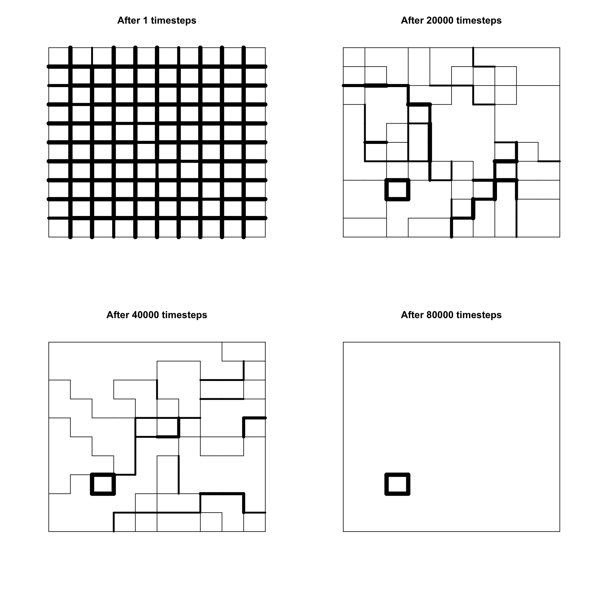
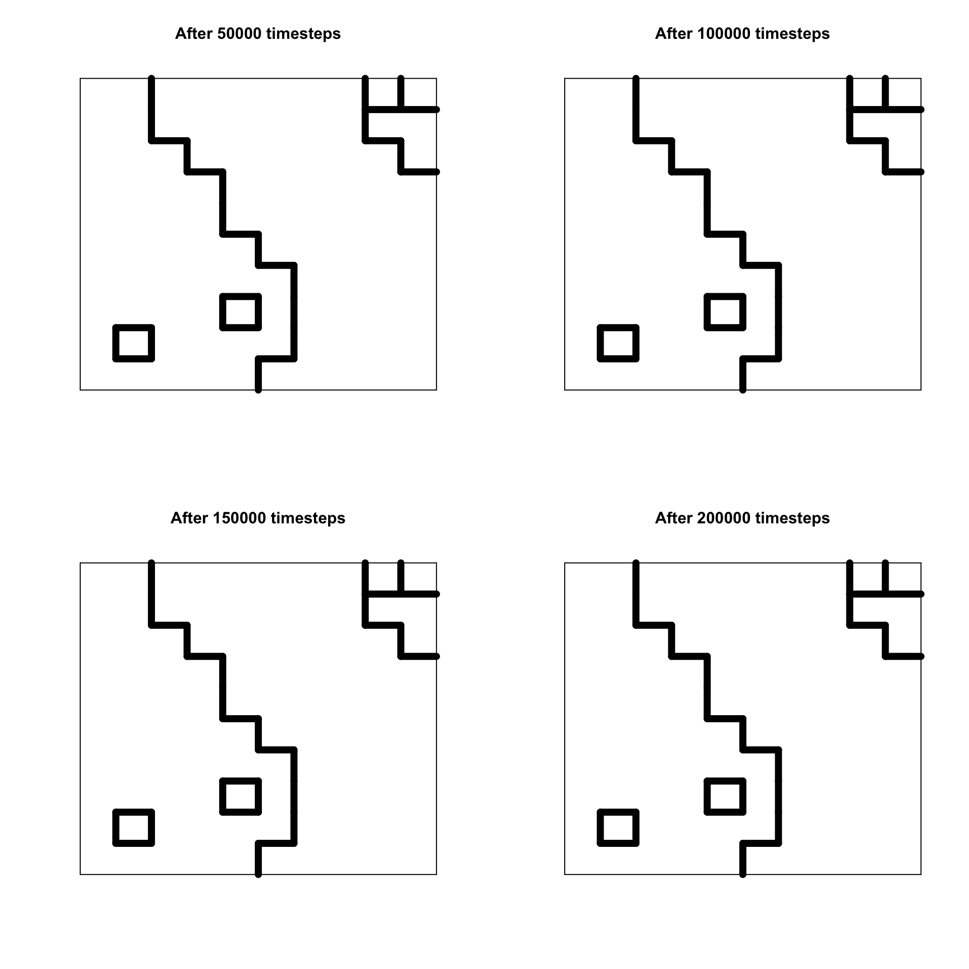
It is likely that by \(t = 80000\) the population has reached stability. This means that all neighbours of every agent are either culturally identical (indicated in the plot by no lines) or maximally culturally dissimilar (indicated by the thickest lines). In both of these cases, no further change can occur. Let’s run the simulation for more timesteps. It should be guaranteed to reach stability by \(t = 200000\).
Now let’s vary \(g\), the number of cultural features, to see how this affects the number of stable regions. With \(g = 15\):
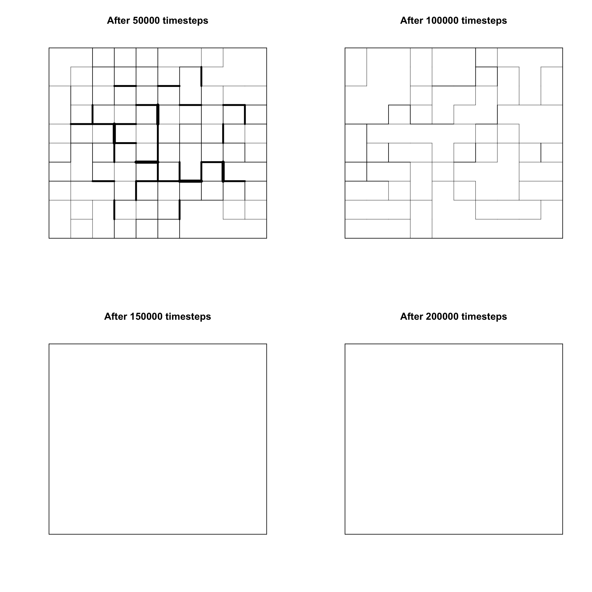
Interestingly, with a larger \(g\) we are almost certain to converge on a single stable region that encompasses the entire grid. What’s more, at \(t = 100000\) there are no highly dissimilar boundaries, only weakly similar ones. This was also observed by Axelrod. Counter-intuitively, having more cultural features increases the likelihood of global homogeneity rather than polarization. This is because with more features, there is a higher chance that two agents will have the same trait value on at least one of those features, and therefore be able to interact and switch traits.
It would be useful to know exactly when a simulation run reaches stability. If a run reaches stability before \(t_{max}\), there is little point continuing the run. We can save time by stopping the simulation at the point at which stability is reached and recording the final agent configuration. We also don’t have to try to guess beforehand when stability might be reached, and risk ending the simulation at \(t_{max}\) before that point.
The following function stability takes an agent matrix as its input and tests whether stability has been reached. The function cycles through each agent (much like in PolarizationPlot, first along rows then along columns), and calculates the similarity of each pair of neighbouring agents. If any of these similarities are greater than zero and less than one, then a variable stable is set to FALSE and the loops are broken using break. Because stable starts out initially TRUE, if the function gets to the end of the cycles without finding a non-stable pair of neighbours, then stable remains TRUE. stable is then outputted from the function at the end.
stability <- function(agent) {

  # cycle thru each agent, compare with neighbours,
  # if similarity >0 and <1 then set stable=false and break the loop(s)

  # retrieve N_side from agent matrix
  N_side <- dim(agent)[1]

  # start with the assumption of stability
  stable <- TRUE

  # cycle thru agents horizontally
  for (Row in 1:N_side) {

    for (Col in 1:(N_side-1)) {

      # agent2 is to the right of agent1
      agent1 <- agent[Row,Col]
      agent2 <- agent[Row,Col+1]

      # make numeric
      agent1 <- as.numeric(unlist(strsplit(agent1, split = NULL)))
      agent2 <- as.numeric(unlist(strsplit(agent2, split = NULL)))

      # get similarity
      similarity <- sum(agent1 == agent2) / length(agent1)

      if (similarity > 0 & similarity < 1) {

        stable <- FALSE
        break

      }
    }

    if (stable == FALSE) break

  }

  # if still possibly stable, cycle vertically
  if (stable == TRUE) {

    for (Row in 1:(N_side-1)) {

      for (Col in 1:N_side) {

        # agent2 is directly below agent1
        agent1 <- agent[Row,Col]
        agent2 <- agent[Row+1,Col]

        # make numeric
        agent1 <- as.numeric(unlist(strsplit(agent1, split = NULL)))
        agent2 <- as.numeric(unlist(strsplit(agent2, split = NULL)))

        # get similarity
        similarity <- sum(agent1 == agent2) / length(agent1)

        if (similarity > 0 & similarity < 1) {

          stable <- FALSE
          break

        }
      }

      if (stable == FALSE) break

    }

  }

  # return stable
  stable

}
Now we can rewrite the Polarization function to add this stability test. We add a new parameter stable_stop to the function definition. When stable_stop is FALSE (the default), Polarization functions as before and continues until \(t_{max}\). When stable_stop is TRUE, then the stability test is activated. At the end of every timestep, the stability function is called. If the returned stable variable is TRUE, then the \(t\) loop is broken. As before, \(t\) is part of the output of the function. While previously this was always \(t_{max}\), now it is the \(t\) at which the simulation reached stability, if stable_stop is TRUE and stability was reached before \(t_{max}\).
Polarization <- function(N_side, g, t_max, stable_stop = FALSE) {

  # make agent matrix of size N_size x N_size
  agent <- matrix(NA,
                  nrow = N_side,
                  ncol = N_side)

  # fill agent with g numbers each a random integer 0-9, stored as chr
  for (n_width in 1:N_side) {

    for (n_height in 1:N_side) {

      agent[n_width,n_height] <- paste(sample.int(10, g, replace = TRUE) - 1,
                                       collapse = "")

    }

  }

  for (t in 1:t_max) {

    # pick a focal agent at random
    focal_row <- sample(1:N_side, 1)
    focal_col <- sample(1:N_side, 1)
    focal <- agent[focal_row, focal_col]

    # pick one of its neighbours at random
    # ignoring non-existent agents outside boundaries

    all_neighbours <- NULL

    if (focal_row-1 >= 1)
      all_neighbours <- append(all_neighbours,
                               agent[focal_row-1, focal_col])
    if (focal_row+1 <= N_side)
      all_neighbours <- append(all_neighbours,
                               agent[focal_row+1, focal_col])
    if (focal_col-1 >= 1)
      all_neighbours <- append(all_neighbours,
                               agent[focal_row, focal_col-1])
    if (focal_col+1 <= N_side)
      all_neighbours <- append(all_neighbours,
                               agent[focal_row, focal_col+1])

    neighbour <- sample(all_neighbours, 1)

    # compare focal and neighbour agents:
    # if there's at least one dissimilar trait,
    # and with prob equal to the similarity between focal and neighbout,
    # set a random dissimilar focal trait to that of the neighbour's

    # separate out traits and make them numeric, for comparing
    focal <- as.numeric(unlist(strsplit(focal, split = NULL)))
    neighbour <- as.numeric(unlist(strsplit(neighbour, split = NULL)))

    # get similarity
    similarity <- sum(focal == neighbour) / length(focal)

    if (similarity > 0 & similarity < 1) {

      if (runif(1) < similarity) {

        if (sum(focal != neighbour) == 1) {
          feature <- which(focal != neighbour)
        } else {
          feature <- sample(which(focal != neighbour), 1)
        }

        focal[feature] <- neighbour[feature]

        agent[focal_row, focal_col] <- paste(focal, collapse = "")

      }

    }

    # if stable_stop is TRUE, break the t-loop if stability is reached
    if (stable_stop) {
      stable <- stability(agent)
      if (stable) break
    }

  }

  # output agent matrix and t
  list(agent = agent, t = t)

}
Running Polarization with stable_stop = TRUE and a very large \(t_{max} = 1000000\) reveals that stability is reached long before this point, most likely less than 100000 timesteps.
data_model <- Polarization(N_side = 10,
                           g = 5,
                           t_max = 1000000,
                           stable_stop = TRUE)

data_model$agent
## [,1] [,2] [,3] [,4] [,5] [,6] [,7] [,8] [,9] [,10]
## [1,] "92469" "92469" "92469" "92469" "92469" "92469" "50820" "50820" "50820" "21656"
## [2,] "17821" "92469" "92469" "92469" "92469" "92469" "92469" "92469" "50820" "50820"
## [3,] "92469" "92469" "92469" "92469" "92469" "92469" "92469" "92469" "92469" "50820"
## [4,] "92469" "92469" "92469" "92469" "92469" "92469" "92469" "92469" "92469" "92469"
## [5,] "92469" "92469" "92469" "92469" "92469" "92469" "92469" "92469" "92469" "92469"
## [6,] "92469" "92469" "92469" "92469" "92469" "92469" "92469" "92469" "92469" "92469"
## [7,] "92469" "92469" "92469" "92469" "92469" "92469" "92469" "92469" "92469" "92469"
## [8,] "92469" "92469" "92469" "92469" "92469" "92469" "92469" "92469" "92469" "92469"
## [9,] "92469" "92469" "92469" "92469" "92469" "18696" "92469" "92469" "92469" "92469"
## [10,] "92469" "92469" "92469" "92469" "92469" "92469" "92469" "92469" "92469" "92469"## [1] 110179Now we have a more nimble simulation, we can systematically vary parameters and measure the effect on the average number of stable regions across multiple runs. The code below runs Polarization for \(g = 5\), \(g = 10\) and \(g = 15\), each for \(r_{max} = 10\) independent runs. The output, both the number of stable regions at stability and the number of timesteps at which this was reached, is recorded in a dataframe called g_analysis. As in previous models, we add the values of each run to a running total then divide by \(r_{max}\) at the end. Finally, because it can take a while to run, we add progress messages using the cat function. This tells us which \(g\) value and which run the simulation is currently at. While this is largely cosmetic, it can be useful to know that a simulation is still running and hasn’t hung up, and how long it might take to finish so you know whether you have time to go get a cup of tea.
g_values <- c(5, 10, 15)

r_max <- 10

g_analysis <- data.frame(cultural_features = g_values,
                         stable_regions = 0,
                         timesteps = 0)

for (g in 1:length(g_values)) {

  cat("Running g =", g_values[g], fill=T)

  for (r in 1:r_max) {

    cat("...Run", r, "of", r_max, fill=T)

    data_model10 <- Polarization(N_side = 10,
                                 g = g_values[g],
                                 t_max = 1000000,
                                 stable_stop = TRUE)

    g_analysis$stable_regions[g] <- g_analysis$stable_regions[g] +
      length(unique(as.vector(data_model10$agent)))

    g_analysis$timesteps[g] <- g_analysis$timesteps[g] +
      data_model10$t

  }

}
## Running g = 5
## ...Run 1 of 10
## ...Run 2 of 10
## ...Run 3 of 10
## ...Run 4 of 10
## ...Run 5 of 10
## ...Run 6 of 10
## ...Run 7 of 10
## ...Run 8 of 10
## ...Run 9 of 10
## ...Run 10 of 10
## Running g = 10
## ...Run 1 of 10
## ...Run 2 of 10
## ...Run 3 of 10
## ...Run 4 of 10
## ...Run 5 of 10
## ...Run 6 of 10
## ...Run 7 of 10
## ...Run 8 of 10
## ...Run 9 of 10
## ...Run 10 of 10
## Running g = 15
## ...Run 1 of 10
## ...Run 2 of 10
## ...Run 3 of 10
## ...Run 4 of 10
## ...Run 5 of 10
## ...Run 6 of 10
## ...Run 7 of 10
## ...Run 8 of 10
## ...Run 9 of 10
## ...Run 10 of 10g_analysis$stable_regions <- g_analysis$stable_regions / r_max
g_analysis$timesteps <- g_analysis$timesteps / r_max
g_analysis## cultural_features stable_regions timesteps
## 1 5 4.8 70513.0
## 2 10 1.0 108668.7
## 3 15 1.0 123129.8The stable_regions column in the g_values dataframe should show that when there are five cultural features (\(g = 5\)), there is more than one stable region, i.e. polarization. When there are ten or fifteen features, there is a single stable region, i.e. homogeneity. This matches the middle column of Axelrod’s Table 2, for 10 traits per feature (Axelrod found a mean of 3.2 stable regions for \(g = 5\), and 1.0 for \(g = 10\) and \(g = 15\)). The timesteps column in g_values reassures us that stability was reached, because they are all much less than the \(t_{max}\) value that was defined.
Summary
The notable feature of Model 10, a replication of Axelrod (1997), is the apparent contradiction between the local interactions of agents and the global dynamics of the model. At the local level, individual agents preferentially interact with neighbours who are more culturally similar to themselves. Their only possible action is to become even more similar by adopting their neighbour’s traits with a probability proportional to their similarity. Yet at the global level, we often see the emergence of stark cultural divisions between regional clusters of agents who are maximally different to other clusters.
Global polarization can therefore emerge despite local preferences for cultural convergence. This perhaps gives some insight into real-world polarization, from racial and socio-economic segregation in cities, to the balkanization of regions within states, to political polarization on social media. These socially undesirable patterns may not necessarily be the result of people’s tendencies to denigrate outgroups or make themselves as dissimilar as possible to others. They may instead be a by-product of the benign desire to preferentially assort with culturally similar others, and become even more similar to those similar others. If the latter is true (and such a claim needs to be empirically tested), this may change how we try to tackle such real world social problems.
Interestingly and counter-intuitively, polarization is more likely to be observed when there are fewer cultural features (a smaller \(g\) in the model). One way of avoiding polarization may therefore be to emphasise the many ways in which people differ. There are not just conservatives and liberals, there are conservatives and liberals who are also football fans and enjoy hiking and like romantic comedies and listen to country music. The more features people may assort on, the more likely interactions are to occur. Axelrod (1997) also found that polarization is reduced when (i) agents interact with more agents, i.e. have more neighbours than just the four we simulated in Model 10, and (ii) when territories are larger, i.e. there are more agents overall. Increasing the range of interactions and number of interactants may therefore be another way to reduce polarization.
On the other hand, the alternative outcome of the model is complete cultural homogeneity. This is also often undesirable. Cultural evolution requires variation on which selection for better alternatives can act. No variation means no adaptation. The loss of minority knowledge, customs and traditions leaves societies less culturally rich and less resilient to environmental change. The cause of homogeneity in Model 10 is similar to the assortation from Model 6, but on multiple traits not just one. The outcome is also similar to conformity (Model 5), which similarly causes the cultural majority to subsume the minority. To preserve minority traditions, some way is needed to counter the benign desire to assort with and copy similar others.
Of course, there are many processes missing from this simple model. Cultural mutation would constantly introduce new variation, acting against both homogeneity and polarization (although see Klemm et al. 2005). Inter-regional competition may shift or dissolve the boundaries between stable regions. The cultural features in Model 10 are simply markers of identity; if instead they affected payoffs, then individuals might happily adopt high-payoff traits from otherwise dissimilar others. Agents are fixed in position and stuck with the same neighbours forever, rather than being able to form new links to other agents (see Centola et al. 2007). Real-world cultural evolution is complex, but the value of simple models like Axelrod’s is to better understand the many simple processes that contribute to a messy, complex reality. What’s more, the dynamics of even simple models like this are often counter-intuitive, as we have seen with the emergence of global polarization despite local convergence, and the effect of \(g\).
One programming innovation of Model 10 was using a matrix to simulate agents within a spatially explicit grid. Each agent’s traits were placed in a fixed position in a square matrix. The [row,column] matrix notation was used to retrieve an agent’s position as well as their neighbours with whom they interact. Matrices can be rectangular as well as square, and also one-dimensional (essentially a line of agents). We also modelled multiple cultural traits per agent, specifically \(g\) cultural features each of which could take one of ten values. This goes beyond the one or two traits and trait values of previous models. We encoded these as character variables to preserve the leading zeroes, which would disappear if we used numeric variables. We converted the character to numeric to compare agents and their neighbours. You should use whatever variable type is most appropriate for the task. Some other minor coding tips: first, use break to break out of loops once you know there will be no further change, or once some condition has been fulfilled, to avoid wasting time; second, always make sure that sample is picking from more than one element, never a single element, otherwise things can go wrong; and third, add messages using cat to keep track of the progress of the simulation.
Exercises
Create some code to track the number of unique regions in every timestep, averaged across \(r_{max}\) independent runs. Plot this average value over time. Does the number of unique regions decline steadily over time or show a different pattern?
In the Model 10 simulations, the number of traits per feature is fixed at 10 (the integers 0-9). Axelrod varied this, comparing 10 with 5 and 15. Modify Polarization to make the number of traits per feature a user-defined variable. Run a similar analysis to the g_analysis above, but varying both \(g\) and the number of traits per feature. Use this to replicate all of Axelrod’s Table 2, showing the mean number of stable regions for every combination of five, ten and fifteen features and traits per feature.
Analyse the effect of varying \(N_{side}\), the size of the grid within which agents are placed, and hence the number of agents in the population. Run a similar analysis to the g_analysis above, but varying \(N_{side}\), and keeping \(g = 5\) and fifteen traits per feature. Plot the average number of stable regions against \(N_{side}\) to replicate Axelrod’s Figure 2.
In Polarization we assumed that each agent had at most four neighbours, to the north, south, east and west (agents at edges and corners had fewer). This is known as a von Neumann neighbourhood, after the mathematician and computer scientist John von Neumann. An alternative is to also include the four agents to the north-west, north-east, south-west and south-east. This gives a maximum of eight neighbours (again, agents at edges and corners will have fewer). This is known as a Moore neighbourhood, after the mathematician and computer scientist Edward F Moore. Modify Polarization such that agents have a Moore neighbourhood rather than a von Neumann neighbourhood. Does this increase or decrease the number of stable regions?
Modify Polarization (with either von Neumann or Moore neighbourhoods) such that neighbourhoods wrap around to the other side of the grid. In other words, an agent at the extreme west edge of the grid will have neighbours to the north, east and south as previously, but also a neighbour to the west, which will be the agent in the same row at the extreme east of the grid. Agents in the corners wrap around in both the north-south and east-west axes. Every agent therefore has exactly four neighbours assuming von Neumann neighbourhoods, or exactly eight assuming Moore neighbourhoods. Do overlapping edges increase or decrease the number of stable regions?
Add mutation to Polarization. In each timestep, pick an agent at random, pick one of their features at random, and with a certain probability determined by a user-defined parameter, switch this feature to a different, random trait value. Complete stability will never be reached with mutation, but explore the effect of mutation on the number of approximately stable regions, and the speed with which this approximate stability is reached, compared to the case of no mutation.
References
Axelrod, R. (1997). The dissemination of culture: A model with local convergence and global polarization. Journal of Conflict Resolution, 41(2), 203-226.
Centola, D., Gonzalez-Avella, J. C., Eguiluz, V. M., & San Miguel, M. (2007). Homophily, cultural drift, and the co-evolution of cultural groups. Journal of Conflict Resolution, 51(6), 905-929.
Klemm, K., Eguiluz, V. M., Toral, R., & San Miguel, M. (2005). Globalization, polarization and cultural drift. Journal of Economic Dynamics and Control, 29(1-2), 321-334.