Model 15: Opinion formation
Introduction
The final model in this mini-series of three adds opinion formation to social contagion (Model 13) and social networks (Model 14). We will recreate a model by Salathé & Bonhoeffer (2008) focussing on vaccination beliefs, a topic of considerable real-world importance.
Salathé & Bonhoeffer (2008) note that many countries suffer disease outbreaks despite ready access to vaccines that prevent those diseases. These outbreaks occur due to the spread of anti-vaccine opinions. These opinions cause people to refuse to vaccinate themselves or their children.
Salathé & Bonhoeffer (2008) assume that anti-vaccine opinions spread via social contagion (see Model 13) on small-world social networks (see Model 14). Rather than simple or complex contagion (Model 14), they assume that an individual switches opinion from pro- to anti-vaccine, or from anti- to pro-vaccine, with probability equal to the proportion of connected neighbours who have a dissimilar opinion multiplied by a parameter \(\Omega\) that determines the strength of opinion formation. This is a form of unbiased cultural transmission (see Model 1), but restricted to an agent’s neighbours rather than the entire population.
For example, if pro-vaccine agent \(i\) has ten neighbours connected to them via edges in the small world network, and six of those neighbours are anti-vaccine, then when \(\Omega = 1\) agent \(i\) has a 0.6 chance of becoming anti-vaccine. When \(\Omega = 0.5\) they have a 0.3 chance of flipping, while if \(\Omega = 0\) they never switch opinion. \(\Omega\) therefore generates opinion clustering, with groups of like-minded individuals causing individuals with dissimilar opinions to switch to their view.
Pro-vaccine agents then get vaccinated and become immune, while anti-vaccine agents remain susceptible. A single infected agent is introduced at time \(t = 0\), and infection is allowed to proceed for \(t_{max} = 300\) timesteps. Note that this is now disease contagion rather than social contagion. The question is: how does opinion clustering, determined by \(\Omega\), affect the number of subsequent infections? Model 15 will reveal the answer.
Model 15
First we generate a small world network using the SmallWorld function from Model 14. If you haven’t already got it loaded, it’s repeated below, along with DrawNetwork which it uses.
SmallWorld <- function(N, k, p, draw_plot = TRUE) {
# 1. create empty adjacency matrix
network <- matrix(0, nrow = N, ncol = N, )
# 2. create ring lattice network
for (Row in 1:N) {
# k/2 neighbours to the right
Col <- (Row+1):(Row+k/2)
Col[which(Col > N)] <- Col[which(Col > N)] - N
network[Row, Col] <- 1
# k/2 neighbours to the left
Col <- (Row-k/2):(Row-1)
Col[which(Col < 1)] <- Col[which(Col < 1)] + N
network[Row, Col] <- 1
}
# 3. rewiring via p
for (j in 1:(k/2)) {
for (i in 1:N) {
if (runif(1) < p) {
# pick jth clockwise neighbour
neighbour <- i + j
if (neighbour > N) neighbour <- neighbour - N
# pick random new neighbour, excluding self and duplicate edges
new_neighbour <- which(network[i,] == 0)
new_neighbour <- new_neighbour[new_neighbour != i]
new_neighbour <- sample(new_neighbour, 1)
# remove edge to old neighbour
network[i,neighbour] <- 0
network[neighbour,i] <- 0
# make edge to new neighbour
network[i, new_neighbour] <- 1
network[new_neighbour, i] <- 1
}
}
}
# 4. draw network if draw_network == TRUE
if (draw_plot == TRUE) {
DrawNetwork(network)
}
# output network from function
network
}
DrawNetwork <- function(network) {
# get N from network matrix
N <- ncol(network)
# N agents around the origin in a big circle
plot(NULL,
xlim = c(-5.5,5.5),
ylim = c(-5.5,5.5),
xlab = "",
ylab = "",
axes = FALSE,
asp = 1)
for (i in 1:N) {
points(5*sin((i-1)*2*pi/N), 5*cos((i-1)*2*pi/N),
pch = 16,
cex = 1.2)
}
# lines representing edges
for (i in 1:N) {
for (j in which(network[i,] == 1)) {
lines(x = c(5*sin((i-1)*2*pi/N), 5*sin((j-1)*2*pi/N)),
y = c(5*cos((i-1)*2*pi/N), 5*cos((j-1)*2*pi/N)))
}
}
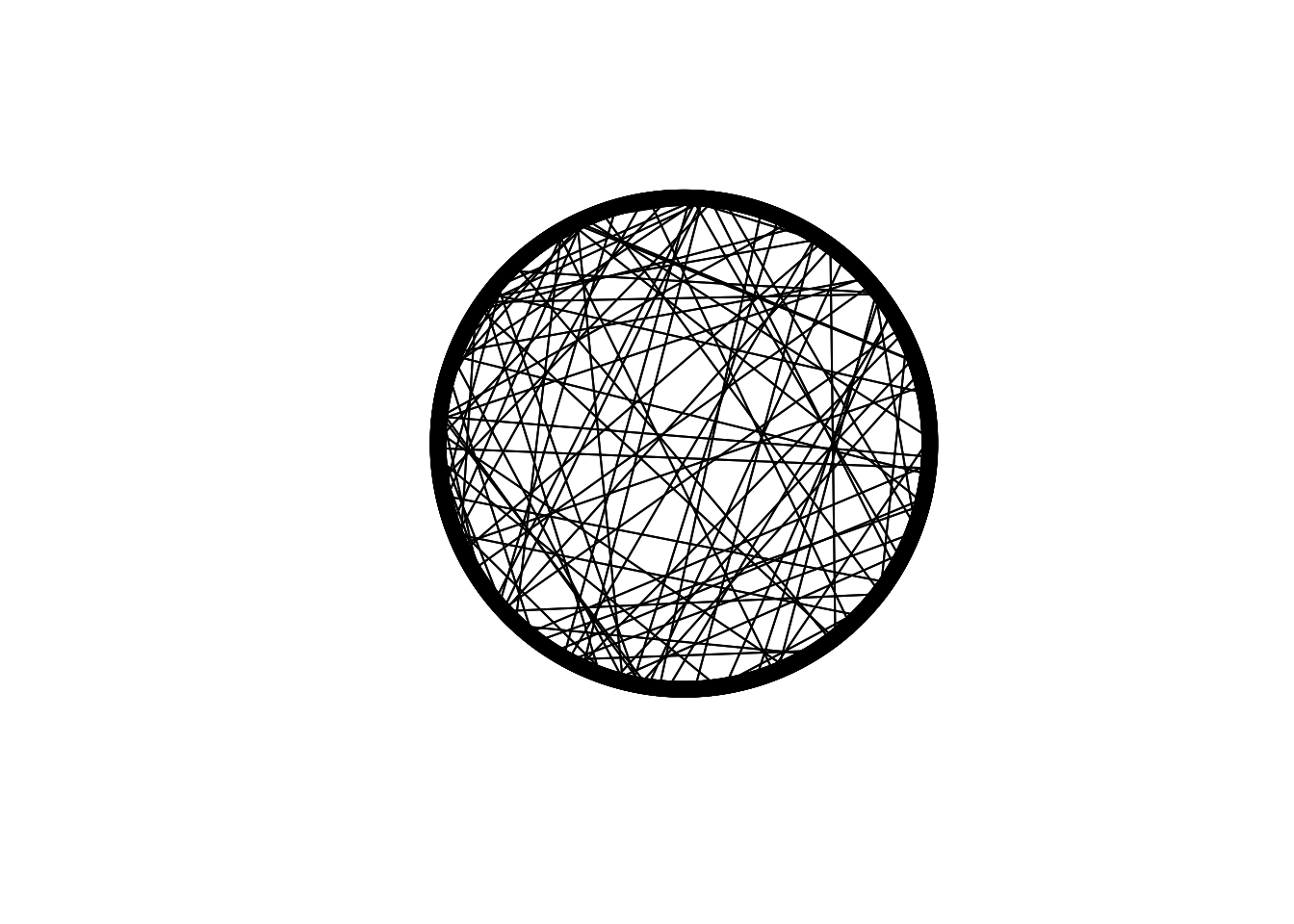
}Salathé & Bonhoeffer (2008) used \(N = 2000\) nodes (i.e. agents) with \(k = 10\) edges (connections) per node and rewiring probability \(p = 0.01\). We create this below, along with a visualisation of the ring lattice network and a 10x10 snippet of the 2000x2000 adjacency matrix to remind us what small world networks look like.
##       [,1] [,2] [,3] [,4] [,5] [,6] [,7] [,8] [,9] [,10]
##  [1,]    0    1    1    1    1    1    0    0    0     0
##  [2,]    1    0    1    1    1    1    1    0    0     0
##  [3,]    1    1    0    1    1    1    1    1    0     0
##  [4,]    1    1    1    0    1    1    1    1    1     0
##  [5,]    1    1    1    1    0    1    1    1    1     1
##  [6,]    1    1    1    1    1    0    1    1    1     1
##  [7,]    0    1    1    1    1    1    0    1    1     1
##  [8,]    0    0    1    1    1    1    1    0    1     1
##  [9,]    0    0    0    1    1    1    1    1    0     1
## [10,]    0    0    0    0    1    1    1    1    1     0
Next we assign opinions to each of the \(N\) agents, stored in a vector opinion. With probability \(c\), agents are pro-vaccine. With probability \(1 - c\) they are anti-vaccine. We use 1 to indicate pro-vaccine, and 0 to indicate anti-vaccine. This is more efficient than using a string such as “pro” or “anti”, and we can get the proportion of pro-vaccination by taking the mean of opinion. We start with \(c = 0.5\), half pro- and half anti-vaccine.
## [1] 0 1 0 1 1 0## [1] 0.488Now we simulate opinion formation, incorporating clustering. First we need to get \(d\), the proportion of an agent’s neighbours who have dissimilar opinions to that agent. Because we’ll need to do this in a few different places in the simulation, we write a function get_d which returns \(d\) for a set of nodes from a network of agents with vaccine-related opinions. The default value of nodes is the entire network, but this can be overridden to get \(d\) for specific nodes, as shown.
get_d <- function(network, opinion, nodes = 1:length(opinion)) {

  d <- rep(NA, length(nodes))

  for (i in nodes) {

    # get i's neighbours from network matrix
    neighbours <- which(network[i,] == 1)

    # proportion with differing opinions
    d[which(nodes == i)] <- sum(opinion[neighbours] != opinion[i]) / length(neighbours)

  }

  # return d
  d

}

get_d(network, opinion, 1)
## [1] 0.5## [1] 0.5000000 0.3636364 0.5555556 0.5000000 0.7000000 0.5000000Right now we need \(d\) for all nodes:
Next we cycle through each node in random order, and for each focal node \(i\), with probability \(d_i \Omega\), node \(i\) switches opinion. This is done with the ifelse command, which is useful for assigning one value if a condition is true, and a different value if it’s false. We set \(\Omega = 1\) so that we can see the effect of clustering later on.
Salathé & Bonhoeffer (2008) made the additional assumption that for every agent that switches (e.g. from pro to anti), another agent switches in the opposite direction (e.g from anti to pro). While artificial, this keeps the proportion of pro- and anti-vaccine agents constant. Consequently, we know that any results we find are due to opinion clustering, rather than overall opinion frequency.
The code below therefore recalculates \(d\) for focal \(i\) and its neighbours (this is where having a function get_d is useful), then repeatedly samples another agent with the same opinion as \(i\) now has, and with probability \(d_j \Omega\) switches \(j\) to \(i\)’s original pre-switch opinion. We then recalculate \(d\) in preparation for the next focal.
omega <- 1

# random order of focal nodes
focal <- sample(N)

for (i in focal) {

  # with prob d*omega
  if (runif(1) < d[i] * omega) {

    # i changes its opinion
    opinion[i] <- ifelse(opinion[i], 0, 1)

    # recalculate d for i and its neighbours
    nodes <- c(i, which(network[i,] == 1))
    d[nodes] <- get_d(network, opinion, nodes)

    # get other nodes with the new opinion, excluding self
    same_opinion <- which(opinion == opinion[i])
    same_opinion <- same_opinion[same_opinion != i]

    # pick a random node j and switch with prob d*omega
    # repeat until successful
    repeat {

      j <- sample(same_opinion, 1)

      if (runif(1) < d[j] * omega) {

        # j changes its opinion
        opinion[j] <- ifelse(opinion[j], 0, 1)

        # recalculate d for j and its neighbours
        nodes <- c(j, which(network[j,] == 1))
        d[nodes] <- get_d(network, opinion, nodes)

        break

      }
    }
  }
}
As a check, we can make sure that the number of pro- vs anti-vaccine agents hasn’t changed:
## [1] 0.488Next we create a vector to store the disease status of each agent. We use the SIR notation from Model 13. All agents are initially susceptible (\(S\)). We then assume that all agents with a pro-vaccine opinion get vaccinated. These agents all become \(R\), for Recovered (this might seem odd given that they never got the disease, but effectively they ‘recovered’ from the vaccine and now cannot become infected, just like someone who recovered from the actual disease and gained natural immunity). Note that \(c\) is therefore not only the probability of pro-vaccine opinions, but also the proportion of the population who are vaccinated and immune.
Next we infect a single random \(S\) individual. The if statement is there in case there are no \(S\) agents, e.g. when \(c = 1\), otherwise we get an error message.
Now we start the t-loop, cycling over \(t_{max} = 300\) timesteps to model the spread (or not) of the infection. Infection occurs for each \(S\) agent with probability \(1 - \exp(-\beta I_n)\), where \(\beta\) is the rate of transmission (fixed at \(\beta = 0.05\)) and \(I_n\) is the number of that agent’s neighbours that are \(I\). Meanwhile, \(I\) nodes recover to become \(R\) with probability \(\gamma = 0.1\) each timestep.
We are interested in tracking the number of infections that occur beyond the ‘patient zero’ that was seeded above. For this we use a vector outbreak to which the number of new infections are added each timestep. Finally, to save cycling through the t-loop pointlessly and wasting time, we add a break clause at the top. If there are either no susceptibles left, or no infecteds left, then the t-loop stops early. Infection cannot occur if there are no susceptibles to become infected, nor if there are no infected agents to infect them.
t_max <- 300
beta <- 0.05
gamma <- 0.1
outbreak <- 0
# start t-loop
for (t in 1:t_max) {
# if no susceptibles or infecteds left, break the loop
if (!any(agent == "S") | !any(agent == "I")) break
# get I_n, number of S's infected neighbours
susceptibles <- which(agent == "S")
I_n <- rep(NA, length(susceptibles))
for (i in 1:length(susceptibles)) {
neighbours <- which(network[susceptibles[i],] == 1)
I_n[i] <- sum(agent[neighbours] == "I")
}
# probability of infection
prob_infection <- 1 - exp(-beta * I_n)
# probs to compare
prob <- runif(length(susceptibles))
# S agents are infected with prob_infection
agent[agent == "S"][prob < prob_infection] <- "I"
# record number of these follow-up infections
outbreak <- outbreak + sum(prob < prob_infection)
# recovery with prob gamma
prob <- runif(sum(agent == "I"))
agent[agent == "I"][prob < gamma] <- "R"
}How many additional infections were there?
## [1] 19This number will vary from simulation to simulation, but with \(c = 0.5\) (a low vaccination rate) and \(\Omega = 1\) (maximum clustering) it is hopefully greater than zero, and perhaps greater than the threshold of 10 that Salathé & Bonhoeffer (2008) required to declare an ‘outbreak’.
We would obviously like to run multiple simulations with the same parameters to obtain a distribution of outbreak values, rather than just one. The following function OpinionFormation wraps all the above code within an r-loop repeated \(r_{max}\) times. Now outbreak stores \(r_{max}\) values rather than just one. To make OpinionFormation standalone, we include SmallWorld and get_d at the beginning.
OpinionFormation <- function(N = 2000,
k = 10,
p = 0.01,
c,
omega,
t_max = 300,
r_max,
beta = 0.05,
gamma = 0.1) {
# define functions
SmallWorld <- function(N, k, p, draw_plot = TRUE) {
# 1. create empty adjacency matrix
network <- matrix(0, nrow = N, ncol = N, )
# 2. create ring lattice network
for (Row in 1:N) {
# k/2 neighbours to the right
Col <- (Row+1):(Row+k/2)
Col[which(Col > N)] <- Col[which(Col > N)] - N
network[Row, Col] <- 1
# k/2 neighbours to the left
Col <- (Row-k/2):(Row-1)
Col[which(Col < 1)] <- Col[which(Col < 1)] + N
network[Row, Col] <- 1
}
# 3. rewiring via p
for (j in 1:(k/2)) {
for (i in 1:N) {
if (runif(1) < p) {
# pick jth clockwise neighbour
neighbour <- i + j
if (neighbour > N) neighbour <- neighbour - N
# pick random new neighbour, excluding self and duplicate edges
new_neighbour <- which(network[i,] == 0)
new_neighbour <- new_neighbour[new_neighbour != i]
new_neighbour <- sample(new_neighbour, 1)
# remove edge to old neighbour
network[i,neighbour] <- 0
network[neighbour,i] <- 0
# make edge to new neighbour
network[i, new_neighbour] <- 1
network[new_neighbour, i] <- 1
}
}
}
# 4. draw network if draw_network == TRUE
if (draw_plot == TRUE) {
DrawNetwork(network)
}
# output network from function
network
}
get_d <- function(network, opinion, nodes = 1:length(opinion)) {
d <- rep(NA, length(nodes))
for (i in nodes) {
# get i's neighbours from network matrix
neighbours <- which(network[i,] == 1)
# proportion with differing opinions
d[which(nodes == i)] <- sum(opinion[neighbours] != opinion[i]) / length(neighbours)
}
# return d
d
}
# initialise output: number of follow-up infections
outbreak <- rep(0, r_max)
# begin r loop:
for (r in 1:r_max) {
# 1. network generation
network <- SmallWorld(N, k, p, draw_plot = FALSE)
# 2. assignment of vaccination opinion
opinion <- sample(c(1,0), N, prob = c(c,1-c), replace = T)
# 3. opinion formation
# skip if omega==0, as no opinion change is possible
if (omega > 0) {
# get d, proportion of differing neighbouring opinions
d <- get_d(network, opinion)
# random order of focal nodes
focal <- sample(N)
for (i in focal) {
# with prob d*omega
if (runif(1) < d[i] * omega) {
# i changes its opinion
opinion[i] <- ifelse(opinion[i], 0, 1)
# recalculate d for i and its neighbours
nodes <- c(i, which(network[i,] == 1))
d[nodes] <- get_d(network, opinion, nodes)
# get other nodes with the new opinion, excluding self
same_opinion <- which(opinion == opinion[i])
same_opinion <- same_opinion[same_opinion != i]
# pick a random node j and switch with prob d*omega
# repeat until successful
repeat {
j <- sample(same_opinion, 1)
if (runif(1) < d[j] * omega) {
# j changes its opinion
opinion[j] <- ifelse(opinion[j], 0, 1)
# recalculate d for j and its neighbours
nodes <- c(j, which(network[j,] == 1))
d[nodes] <- get_d(network, opinion, nodes)
break
}
}
}
}
}
# 4. vaccination according to opinion
agent <- rep("S", N)

agent[opinion == 1] <- "R"
# 5. infection of a random susceptible individual (if any are present)
if (any(agent == "S")) {

      agent[sample(which(agent == "S"), 1)] <- "I"

}
# 6. spread of infection
# start t-loop
for (t in 1:t_max) {
# if no susceptibles or infecteds left, break the loop
if (!any(agent == "S") | !any(agent == "I")) break
# get I_n, number of S's infected neighbours
susceptibles <- which(agent == "S")
I_n <- rep(NA, length(susceptibles))
for (i in 1:length(susceptibles)) {
neighbours <- which(network[susceptibles[i],] == 1)
I_n[i] <- sum(agent[neighbours] == "I")
}
# probability of infection
prob_infection <- 1 - exp(-beta * I_n)
# probs to compare
prob <- runif(length(susceptibles))
# S agents are infected with prob_infection
agent[agent == "S"][prob < prob_infection] <- "I"
# record number of these follow-up infections
outbreak[r] <- outbreak[r] + sum(prob < prob_infection)
# recovery with prob gamma
prob <- runif(sum(agent == "I"))
agent[agent == "I"][prob < gamma] <- "R"
}
}
# export outbreak
outbreak
}Note that all parameters except \(c\) and \(\Omega\) are set to the default values that Salathé & Bonhoeffer (2008) used and did not change. Also \(r_{max}\), as their \(r_{max} = 2000\) can lead to long simulation times. With \(c = 0.5\), \(\Omega = 1\) and \(r_{max} = 100\):
data_model15 <- OpinionFormation(c = 0.5, omega = 1, r_max = 100)

# histogram of infections
hist(data_model15,
     main = "",
     xlab = "number of infections")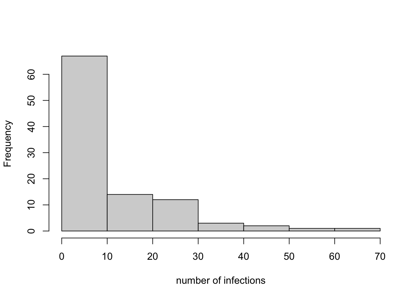
## [1] 10.42## [1] 0.37The histogram shows a range of infection frequencies across the 100 runs, most commonly zero or near to zero, and less frequently greater than 10. The mean number of infections is 10.42, and 0.37 of the runs count as ‘outbreaks’ according to Salathé & Bonhoeffer (2008). This should be similar to the value of 0.4 found by Salathé & Bonhoeffer (2008; Figure 1c), although not exactly because they ran 2000 simulations rather than 100.
We can complete the recreation of Salathé & Bonhoeffer’s Figure 1c by running simulations for a range of values of \(c\), each of which is repeated for \(\Omega = 0\) and \(\Omega = 1\).
c_values <- seq(0.5,0.95,0.05)
omega_values <- c(0,1)
infections <- NULL
r_max <- 100

for (omega in omega_values) {

  for (c in c_values) {

    infections <- append(infections,
                         OpinionFormation(c = c,
                                          omega = omega,
                                          r_max = r_max))

  }

}

# create dataframe for barplot
bar_data <- data.frame(omega = rep(omega_values, each = r_max*length(c_values)),
                       c = rep(c_values, each = r_max),
                       infections)

# reformat based on outbreaks (>=10 infections)
bar_data <- by(bar_data$infections >= 10,
               list(bar_data$omega, bar_data$c*100),
               FUN = sum) / r_max

# plot barplot
barplot(bar_data,
        ylab = "outbreak probability",
        xlab = "vaccination coverage (%)",
        beside = TRUE,
        legend.text = c("unclustered", "clustered"))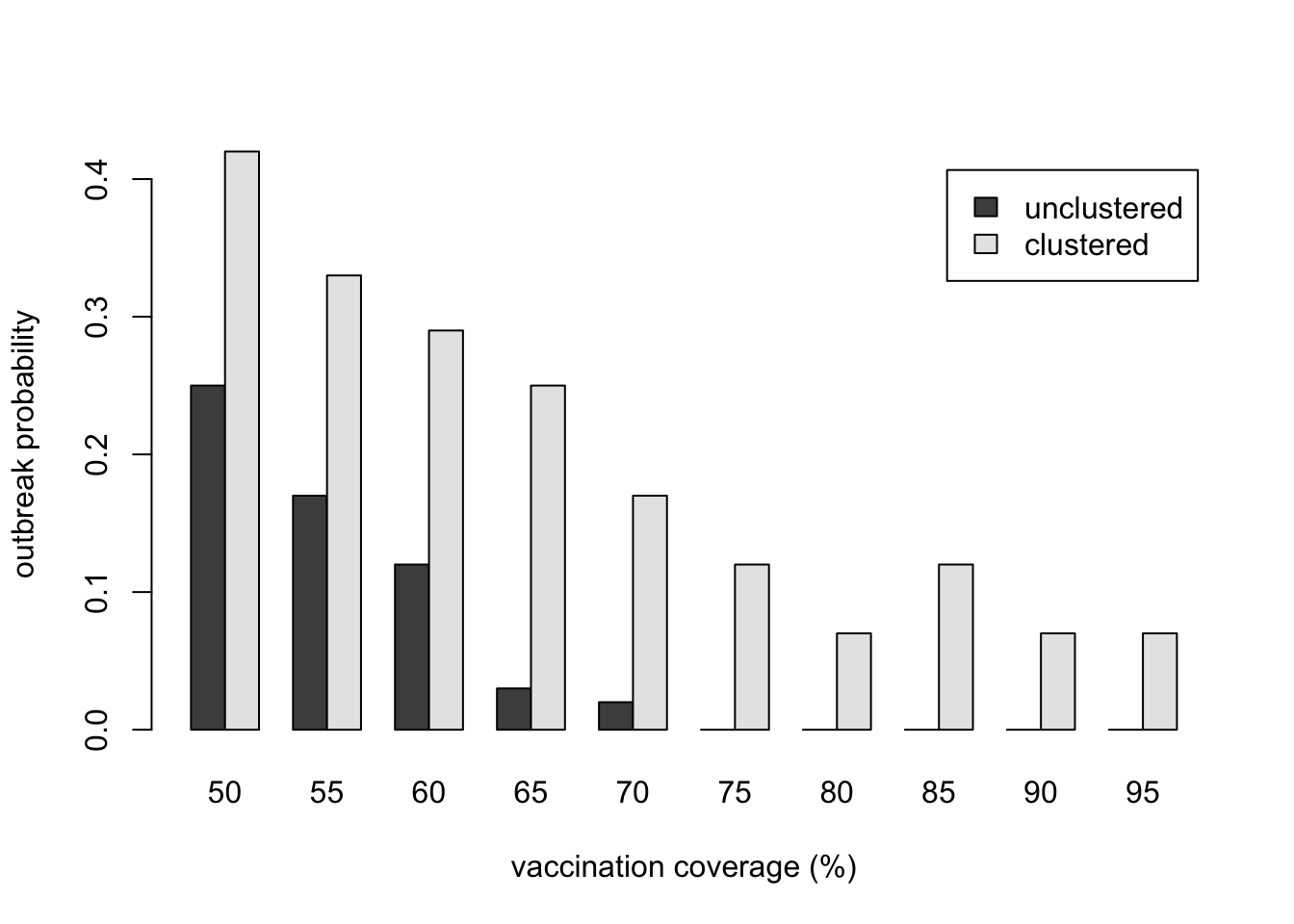
Here we have recreated Salathé & Bonhoeffer’s Figure 1c, albeit less perfectly given our smaller number of runs. The result should be qualitatively the same, however: outbreaks are less likely with greater vaccination coverage (larger \(c\)), but for each value of \(c\), outbreaks are more likely when there is opinion clustering (\(\Omega = 1\)) than with no opinion clustering (\(\Omega = 0\)). At high levels of vaccination (>80%), an unclustered population has achieved herd immunity, whereas a clustered population still suffers outbreaks.
Summary
Model 15 recreated an important model of Salathé & Bonhoeffer (2008). This model combined unbiased transmission (Model 1), SIR contagion models (Model 13) and small world social networks (Model 14) to explore the effect of vaccine-related opinion clustering on the spread of diseases. Agents switch opinion, from pro- to anti-vaccine or anti- to pro-vaccine, in proportion to the number of neighbours who have dissimilar opinions, a form of unbiased cultural transmission. The clear finding is that opinion clustering increases the number of infections and makes outbreaks more likely, compared to a lack of clustering.
This finding has implications for controlling diseases for which vaccines are available. This is a timely topic given the global covid pandemic, as well as previous outbreaks caused by vaccine refusal such as MMR in the UK. People do not get their opinions from random others. They get them from their friends, family, neighbours and work colleagues. This generates self-reinforcing clusters of anti-vaccine opinions, and consequently disease outbreaks. Spending billions of pounds on vaccine development is pointless if anti-vaccine opinions mean that large clusters of people refuse to take it. Models like Salathé & Bonhoeffer’s are important for suggesting interventions that might prevent opinion clustering, or break up clusters that have already formed. See Funk et al. (2010) for further discussion.
In terms of programming, we again saw the advantage of using functions. The previous function SmallWorld was re-used, and a new function get_d was created and used several times, preventing the repetition of the same code in different places. We also made use of the break command to speed up the simulation. If there are instances when you know nothing further will happen, such as when there are no Susceptibles left to be infected or Infecteds left to infect them, use break to exit the loop and save time.
Exercises
Recreate Salathé & Bonhoeffer’s Figure 1b, showing the increase in outbreak probability for different values of \(c\) and \(\Omega\).
Modify OpinionFormation to plot the frequency of \(I\), \(S\) and \(R\) over time as we did in Model 13. Examine the trajectories for different combinations of \(c\) and \(\Omega\).
Salathé & Bonhoeffer (2008) only varied \(c\) and \(\Omega\). Explore the effect on the number of infections of varying the other parameters: \(N\), \(k\), \(p\), \(\beta\) and \(\gamma\).
In real life, vaccination opinion is likely to be continuous rather than dichotomous. Rewrite OpinionFormation so that opinion is a probability from 0 to 1 specifying the likelihood that an agent gets vaccinated. Think about how to implement \(c\), the probability of being pro-vaccine (e.g. as a distribution rather than a single probability), and \(d\), now that neighbours will be unlikely to ever have an identical opinion (e.g. as a blending rule from Model 8).
Rewrite OpinionFormation replacing the \(d_i \Omega\) switching rule with (i) simple contagion, where just one dissimilar neighbour causes opinion change; (ii) complex contagion, where a threshold of two or more neighbours are needed to cause opinion change; (iii) conformity, following Model 5, where agents adopt the majority opinion amongst its neighbours; and (iv) prestige bias, in which one or more agents are designated as ‘celebrities’ and have a disproportionate influence on their neighbour’s opinions. How do the number of infections generated by these transmission assumptions differ from Salathé & Bonhoeffer’s (2008) original transmission rule?
References
Funk, S., Salathé, M., & Jansen, V. A. (2010). Modelling the influence of human behaviour on the spread of infectious diseases: a review. Journal of the Royal Society Interface, 7(50), 1247-1256.
Salathé, M., & Bonhoeffer, S. (2008). The effect of opinion clustering on disease outbreaks. Journal of The Royal Society Interface, 5(29), 1505-1508.