Model 3: Biased transmission (direct / content bias)
Introduction
So far we have looked at unbiased transmission (Model 1) and unbiased/biased mutation (Model 2). Let’s complete the set by looking at biased transmission. This occurs when one trait or one demonstrator is more likely to be copied than another trait or demonstrator. Trait-based copying is often called ‘direct’ or ‘content’ bias, while demonstrator-based copying is often called ‘indirect’ or ‘context’ bias. Both are sometimes also called ‘cultural selection’ because one thing (trait or demonstrator) is selected to be copied over another. In Model 3 we’ll look at trait-based (direct, content) bias.
(As an aside, there is a confusing array of terminology in the field of cultural evolution, as illustrated by the preceding paragraph. That’s why models are so useful. Words and verbal descriptions can be ambiguous. Often the writer doesn’t realise that there are hidden assumptions or unrecognised ambiguities in their descriptions. They may not realise that what they mean by ‘cultural selection’ is entirely different to how someone else uses it. Models are great because they force us to specify exactly what we mean by a particular term or process. I can use the words in the paragraph above to describe biased transmission, but it’s only really clear when I model it, making all my assumptions explicit.)
Model 3
As in Model 1 and Model 2, we assume there are two traits \(A\) and \(B\). Let’s assume that biased transmission favours trait \(A\). Perhaps \(A\) is a more effective tool, more memorable story, or more easily pronounced word. We’re not including any mutation in the model, so we need to include some \(A\)s at the beginning of the simulation otherwise it would never appear. However, let’s make it initially rare. Then we can see how selection favours this initially-rare trait.
To simulate biased transmission, following Model 1, we assume that each agent chooses another agent from the previous generation at random. But this time, if that chosen agent possesses trait \(A\), then the focal agent copies trait \(A\) with probability \(s\). This parameter \(s\) gives the strength of biased transmission, or the probability that an agent encountering another agent with a more favourable trait than their current trait abandons their current trait and adopts the new trait. If \(s = 0\), there is no selection and agents never switch as a result of biased transmission. If \(s = 1\), then agents always switch when encountering a favoured alternative.
Below is a function BiasedTransmission that implements all of these processes.
BiasedTransmission <- function (N, s, p_0, t_max, r_max) {

  # create a matrix with t_max rows and r_max columns, fill with NAs, convert to dataframe
  output <- as.data.frame(matrix(NA, t_max, r_max))

  # purely cosmetic: rename the columns with run1, run2 etc.
  names(output) <- paste("run", 1:r_max, sep="")

  for (r in 1:r_max) {

    # create first generation
    agent <- data.frame(trait = sample(c("A","B"), N, replace = TRUE,
                        prob = c(p_0,1-p_0)))

    # add first generation's p to first row of column r
    output[1,r] <- sum(agent$trait == "A") / N

    for (t in 2:t_max) {

      # biased transmission

      # copy agent to previous_agent dataframe
      previous_agent <- agent

      # for each agent, pick a random agent from the previous generation
      # as demonstrator and store their trait
      demonstrator_trait <- sample(previous_agent$trait, N, replace = TRUE)

      # get N random numbers each between 0 and 1
      copy <- runif(N)

      # if demonstrator has A and with probability s, copy A from demonstrator
      agent$trait[demonstrator_trait == "A" & copy < s] <- "A"

      # get p and put it into output slot for this generation t and run r
      output[t,r] <- sum(agent$trait == "A") / N

    }

  }

  # first plot a thick line for the mean p
  plot(rowMeans(output),
       type = 'l',
       ylab = "p, proportion of agents with trait A",
       xlab = "generation",
       ylim = c(0,1),
       lwd = 3,
       main = paste("N = ", N, ", s = ", s, sep = ""))

  for (r in 1:r_max) {

    # add lines for each run, up to r_max
    lines(output[,r], type = 'l')

  }

  output  # export data from function
}
Most of BiasedTransmission is recycled from Model 1 and Model 2. As before, we set up a dataframe to hold the output from multiple runs, and in generation \(t = 1\) create a dataframe to hold the trait of each agent. The plot function is also similar, but now we add \(s\) to the plot title so we don’t forget it.
The major change is that we now include biased transmission from the second generation onwards. Using vectorised code, we pick for each of \(N\) agents one of the previous generation’s agents at random and store their trait in demonstrator_trait. Then we get random numbers between 0 and 1 for each agent and store these in copy. If the demonstrator has trait \(A\) (demonstrator_trait == “A”), and with probability \(s\) (copy < s), then the agent adopts trait \(A\).
Let’s run our BiasedTransmission model. Remember we are starting with a population with a small number of \(A\)s, so \(p_0 = 0.01\).
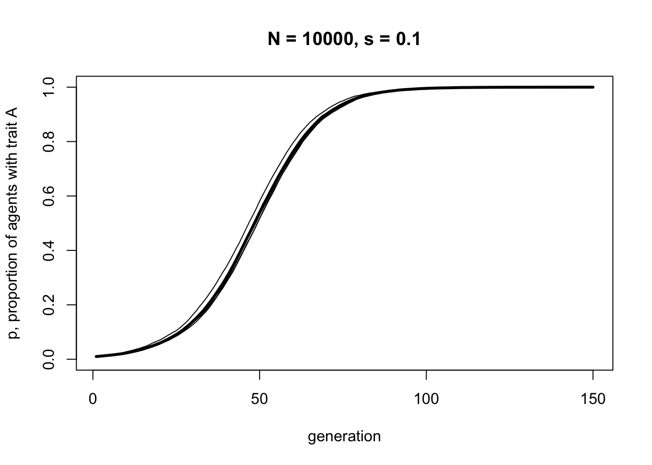
With a moderate selection strength of \(s = 0.1\), we can see that \(A\) gradually replaces \(B\) and goes to fixation. It does this in a characteristic manner: the increase is slow at first, then picks up speed, then plateaus.
Note the difference to biased mutation. Where biased mutation was r-shaped, with a steep initial increase, biased transmission is s-shaped, with an initial slow uptake. This is because the strength of biased transmission, like selection in general, is proportional to the variation in the population. When \(A\) is rare initially, there is only a small chance of picking another agent with \(A\). As \(A\) spreads, the chances of picking an \(A\) agent increases. As \(A\) becomes very common, there are few \(B\) agents left to switch.
Let’s double the selection strength to \(s = 0.2\), below.
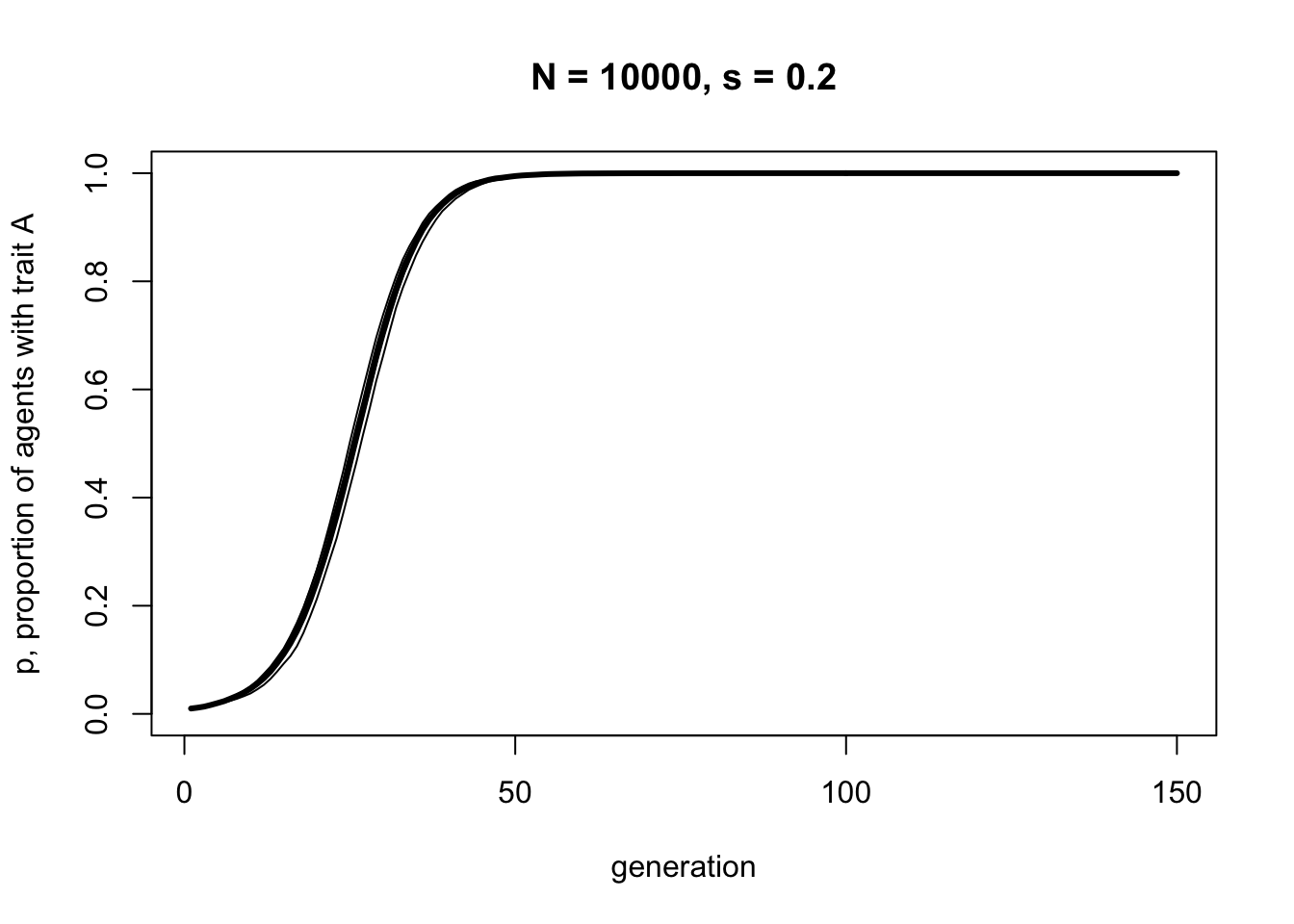
As we might expect, increasing the strength of selection increases the speed with which \(A\) goes to fixation. Note, though, that it retains the s-shape.
Summary
In Model 3 we saw how biased transmission causes a trait favoured by the selection bias to spread and go to fixation in a population, even when it is initially very rare. Biased transmission differs in its dynamics from biased mutation. Its action is proportional to the variation in the population at the time at which it acts. It is strongest when there is lots of variation (in our model, when there are equal numbers of \(A\) and \(B\) at \(p = 0.5\)), and weakest when there is little variation (when \(p\) is close to 0 or 1). This generates an s-shaped pattern of diffusion over time.
S-shaped diffusion curves like the ones we generated using Model 3 are ubiquitous in the real world. Rogers (2010) catalogued numerous examples of the s-shaped diffusion of novel technological and social innovations, from the spread of hybrid seed corn to the spread of new methods for teaching mathematics. Here is one example at the country level, concerning the spread of postage stamps in different European countries (data from Pemberton 1936):
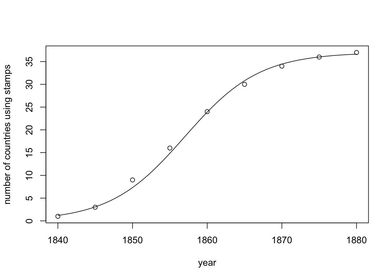
Given that it is unlikely that 37 countries independently invented postage stamps over such a brief period, we can probably attribute the diffusion of postage stamps to a form of biased cultural transmission, as national postal services observed and copied the effective use of stamps in neighbouring countries. Henrich (2001) explicitly linked s-shaped diffusion curves to directly biased cultural transmission, rather than biased mutation, which as we saw in Model 2 generates r-shaped diffusion curves. Similarly, Newberry et al. (2017) provided evidence of s-shaped diffusion curves in the spread of novel grammatical forms, using them to distinguish biased transmission / cultural selection from unbiased transmission (see Model 1). However, we should also be cautious not to jump to conclusions. Many processes generate s-shaped diffusion curves, not just biased transmission, including sometimes purely individual-level biased mutation (Reader 2004; Hoppitt et al. 2010).
Exercises
Try different values of \(s\) to confirm that larger \(s\) increases the speed with which \(A\) goes to fixation.
Change \(s\) in BiasedTransmission to \(s_a\), and add a new parameter \(s_b\) which specifies the probability of an agent copying trait \(B\) from a demonstrator who possesses that trait. Run the simulation to show that the equilibrium value of \(p\), and the speed at which this equilibrium is reached, depends on the difference between \(s_a\) and \(s_b\). How do these dynamics differ from the \(mu_a\) and \(mu_b\) you implemented in Model 2 Q5?
Analytical Appendix
As before, we have \(p\) agents with trait \(A\) and \(1 - p\) agents with trait \(B\). The \(p\) agents with trait \(A\) keep their \(A\)s, because \(A\) is favoured by biased transmission. The \(1 - p\) agents with trait \(B\) pick another agent at random. If the random agent has \(B\) then nothing happens. However if the random agent has \(A\), which they will with probability \(p\), then with probability \(s\) they switch to that trait \(A\). We can therefore write the recursion for \(p\) under biased transmission as:
\[p' = p + p(1-p)s \hspace{30 mm}(3.1)\]
The first term on the right-hand side is the unchanged \(A\) bearers, and the second term is the \(1-p\) \(B\)-bearers who find one of the \(p\) \(A\)-bearers and switch with probability \(s\).
Here is some code to plot this biased transmission recursion:
p <- rep(0, 150)
p[1] <- 0.01
s <- 0.1

for (i in 2:150) {
  p[i] <- p[i-1] + p[i-1]*(1-p[i-1])*s
}

plot(p,
     type = 'l',
     ylab = "p, proportion of agents with trait A",
     xlab = "generation",
     ylim = c(0,1),
     lwd = 3,
     main = paste("s = ", s, sep = ""))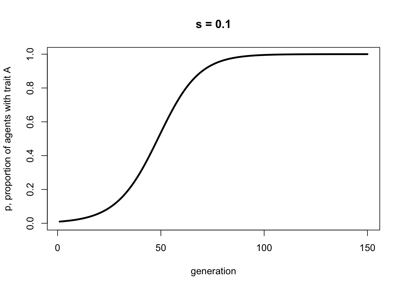
The curve above should be identical to the simulation curve, given that the simulation had the same biased transmission strength \(s\) and a large enough \(N\) to minimise stochasticity.
From Equation 3.1 above, we can see how the strength of biased transmission depends on variation in the population, given that \(p (1 - p)\) is the formula for variance. This determines the shape of the curve, while \(s\) determines the speed with which the equilibrium \(p^*\) is reached.
But what is the equilibrium \(p^*\) here? In fact there are two. As before, the equilibrium can be found by setting the change in \(p\) to zero, or when:
\[p(1-p)s = 0 \hspace{30 mm}(3.2)\]
There are three ways in which the left-hand side can equal zero: when \(p = 0\), when \(p = 1\) and when \(s = 0\). The last case is uninteresting: it would mean that biased transmission is not occurring. The first two cases simply say that if either trait reaches fixation, then it will stay at fixation. This is to be expected, given that we have no mutation in our model. It contrasts with unbiased and biased mutation, where there is only one equilibrium value of \(p\).
We can also say that \(p = 0\) is an unstable equilibrium, meaning that any slight perturbation away from \(p = 0\) moves \(p\) away from that value. This is essentially what we simulated above: a slight perturbation starting at \(p = 0.01\) went all the way up to \(p = 1\). In contrast, \(p = 1\) is a stable equilibrium: any slight perturbation from \(p = 1\) immediately goes back to \(p = 1\).
References
Henrich, J. (2001). Cultural transmission and the diffusion of innovations: Adoption dynamics indicate that biased cultural transmission is the predominate force in behavioral change. American Anthropologist, 103(4), 992-1013.
Hoppitt, W., Kandler, A., Kendal, J. R., & Laland, K. N. (2010). The effect of task structure on diffusion dynamics: Implications for diffusion curve and network-based analyses. Learning & Behavior, 38(3), 243-251.
Newberry, M. G., Ahern, C. A., Clark, R., & Plotkin, J. B. (2017). Detecting evolutionary forces in language change. Nature, 551(7679), 223-226.
Pemberton, H. E. (1936). The curve of culture diffusion rate. American Sociological Review, 1(4), 547-556.
Reader, S. M. (2004). Distinguishing social and asocial learning using diffusion dynamics. Animal Learning & Behavior, 32(1), 90-104.
Rogers, E. M. (2010). Diffusion of innovations. Simon and Schuster.