Model 11: Cultural group selection
Introduction
The evolution of cooperation is a major topic across the biological and social sciences. Cooperation is defined as helping another individual, often at some cost to the helper (costly cooperation is sometimes called ‘altruism’ or ‘altruistic cooperation’). Cooperation is rife in nature, from parents looking after their offspring to sterile worker bees feeding their queen. It also underpins all human societies, from sharing food to paying taxes. Yet altruistic cooperation is a puzzle. All else being equal, a defector (or ‘free-rider’) who never cooperates yet receives help from others will do better than an altruistic cooperator who bears the cost of helping. Consequently, the emergence and maintenance of cooperation requires explanation (West et al. 2007).
This basic free-rider problem applies to the genetic evolution of cooperative behaviour in nature, where costs and benefits are incurred and accrued in the currency of lifetime biological fitness (West et al. 2007). It also applies to human societies where costs and benefits take the form of monetary or other kinds of more immediate payoffs (Apicella & Silk 2019). Examples include taxation systems where free-riding is not paying tax yet benefiting from publicly-funded roads, schools and hospitals, or communal living, where defectors who never wash dishes free-ride on the washing up effort of others. Such systems are characterised by a conflict between the individual and group level: within groups, free-riding individuals do better than cooperating individuals, yet groups of cooperators collectively do better than groups of free-riders. Non-dish-washing free-riders expend less effort than diligent dish-washers yet benefit from using clean dishes washed by others. Yet if everyone free-rides, the dishes quickly pile up.
Solutions to the free-rider problem include kin selection, where cooperators direct help to genetic relatives; reciprocity, where cooperators direct help to others who are likely to return the favour; and punishment, where cooperators punish defectors for not cooperating (West et al. 2007; Apicella & Silk 2019). Yet each of these has limitations with respect to human cooperation: kin selection cannot explain cooperation towards non-kin, which humans do frequently; reciprocity cannot explain cooperation between strangers and breaks down in large groups, which are again common features of human societies; and punishment is itself costly, leading to a second-order free-rider problem where non-punishing cooperators outcompete punishing cooperators.
Consequently, some cultural evolution researchers have suggested that human cooperation can arise via cultural group selection (Richerson et al. 2016). This occurs when more-cooperative groups outcompete less-cooperative groups in between-group competition. Genetic group selection does not seem to work: between-group genetic variation is easily broken down by migration, and individual-level natural selection is too strong. Cultural evolution, however, provides better conditions: rapid cultural selection (Model 3) can generate differences between groups, and processes such as conformity (Model 5) or polarisation (Model 10) can maintain between-group cultural variation despite frequent migration (see Model 7). Between-group competition can occur via direct conquest, e.g. warfare, where more-cooperative societies full of self-sacrificial fighters out-compete less-cooperative societies full of deserting back-stabbers. Or it can occur indirectly, such as where more-cooperative societies, e.g. ones with better social welfare systems, attract more migrants than less-cooperative societies. Success in between-group competition does not necessarily require the death of the defeated group’s members. Instead, defeated group members can disband and join the winning group.
The evolution of cooperation is a highly contentious topic. Verbal arguments often go round in circles because different scholars have different understandings of terms like cooperation, punishment and group selection. This makes formal models crucial for clarifying assumptions and arguments.
Here we will recreate an influential agent-based model of cultural group selection from Boyd, Gintis, Bowles & Richerson (2003). This model features costly (i.e. altruistic) punishment within groups, mixing / migration between groups, payoff-biased social learning and between-group selection. While it is not the only model of cultural group selection, it provides a good example to help understand and evaluate the hypothesis.
Model 11
Let’s introduce the model step by step, with code, before putting it all inside a function. There are \(N\) groups each containing a fixed number of \(n\) individuals. Individuals come in three types, characterised by three different behaviours: cooperators (C), defectors (D) and punishers (P).
As the model is quite complex, we will use matrices instead of dataframes as they are faster. The code below creates a matrix with \(N\) columns, one per group, and \(n\) rows, one per agent, to hold the type (C, D or P). As before, we use [row,column] notation to access a specific agent. For example, agent[3,2] returns the behaviour of the third agent in the second group. For now we assume \(N = 4\) groups with \(n = 4\) agents per group. One group has Cs and Ds, one Ps and Ds, one a mix of all three types, and one all Ds.
N <- 4  # 4 groups
n <- 4  # 4 agents per group

# create agent matrix, each column is a group
# can be C (cooperator), D (defector) or P (punisher)
agent <- matrix(nrow = n, ncol = N)

agent[,1] <- c("C", "C", "D", "D")
agent[,2] <- c("D", "D", "P", "P")
agent[,3] <- c("P", "P", "C", "D")
agent[,4] <- c("D", "D", "D", "D")

agent
## [,1] [,2] [,3] [,4]
## [1,] "C" "D" "P" "D"
## [2,] "C" "D" "P" "D"
## [3,] "D" "P" "C" "D"
## [4,] "D" "P" "D" "D"Now we create a payoff matrix. This has the same structure as agent. Each position in payoff holds the payoff for the individual in the equivalent position in agent. For example, payoff[3,2] holds the payoff of the third agent in group 2. All individuals start with a baseline payoff of 1, from which various costs are subtracted. (NB While this baseline payoff of 1 is not explicitly specified in Boyd et al. 2003, it is needed to avoid negative payoffs. Negative payoffs would mess up subsequent calculations of relative payoffs.)
##      [,1] [,2] [,3] [,4]
## [1,]    1    1    1    1
## [2,]    1    1    1    1
## [3,]    1    1    1    1
## [4,]    1    1    1    1
Now we simulate five stages that occur in each timestep.
Stage 1 is cooperation. Cooperators and punishers cooperate with probability \(1-e\) and defect with probability \(e\). The parameter \(e\) represents errors, where Cs or Ps defect by mistake when they meant to cooperate. For now we will set \(e = 0\) to keep the output the same when you run it, but you can increase it to explore its effect here. We will increase it in the simulations below to \(e = 0.01\).
Cooperation reduces the cooperating agent’s payoff by \(c\). This makes cooperation costly, i.e. altruistic. Defectors always defect and pay no cost. We set \(c = 0.2\), representing a fairly substantial cost.
The following vectorised code implements this. To identify contributors we create a matrix of probabilities, contribute, to compare against \(1 - e\) for each P and C agent. This gives a matrix contributors that is TRUE if the agent contributes and FALSE if they don’t. Contributing agents’ payoffs are then reduced by \(c\). Because \(e = 0\), the matrices will show that all the Ps and Cs pay the cost, and the Ds do not. At this stage, defection pays.
e <- 0  # cooperation error rate
c <- 0.2  # cost of cooperation

# probs for contribution (1-e)
contribute <- matrix(runif(n*N), nrow = n, ncol = N)

# contributors are Ps or Cs with prob 1-e
contributors <- (agent == "P" | agent == "C") & contribute > e

# reduce payoffs of contributing Ps and Cs by c
payoff[contributors] <- payoff[contributors] - c

contributors
## [,1] [,2] [,3] [,4]
## [1,] TRUE FALSE TRUE FALSE
## [2,] TRUE FALSE TRUE FALSE
## [3,] FALSE TRUE TRUE FALSE
## [4,] FALSE TRUE FALSE FALSE## [,1] [,2] [,3] [,4]
## [1,] 0.8 1.0 0.8 1
## [2,] 0.8 1.0 0.8 1
## [3,] 1.0 0.8 0.8 1
## [4,] 1.0 0.8 1.0 1Stage 2 is punishment. Punishers (Ps) punish every agent in their group who defected in the first stage. Punishment reduces each punished agent’s payoff by \(p/n\) at a cost of \(k/n\) to the punisher. The parameter \(k\) makes punishment costly, i.e. altruistic.
Note that punishment scales with the number of defectors: the more punishers there are in a group, the more punishment defectors receive. The more defectors there are, the more costly punishment is to the punisher. We set \(p = 0.8\) and \(k = 0.2\) such that punishment is more costly for the punished than the punisher. For example, the cost of burning down someone’s house is less than the cost of having your house burned down.
In the following code, we first identify groups that have at least one P using Pgroups. We only need to apply our punishment routine to these groups. This saves a bit of time. Then we get a matrix of defections, those agents who are D or who are P or C with probability \(e\). Then we cycle through each agent \(i\) of each punishment group \(j\) using two for loops. For each punishing agent, we reduce the punisher’s payoff by \(k/n\) per defector in their group, and each defector’s payoff by \(p/n\). Note that to get all group members except the focal individual, we use the negative sign. For example, payoff[-i,j] returns all payoffs of agents in group \(j\) who are not \(i\).
p <- 0.8  # cost to punished
k <- 0.2  # cost to punisher

# columns/groups with at least one P
Pgroups <- unique(which(agent=="P", arr.ind=TRUE)[,"col"])

# defections (Ds and Ps/Cs with probability e)
defections <- agent == "D" | ((agent == "P" | agent == "C") & contribute <= e)

# cycle thru Pgroups (j) and agents (i)
for (j in Pgroups) {

  for (i in 1:n) {

    # if the agent is P
    if (agent[i,j] == "P") {

      # reduce punisher's payoff by k/n per defection
      payoff[i,j] <- payoff[i,j] - sum(defections[-i,j]) * k / n

      # reduce each defector's payoff by p/n
      payoff[-i,j][defections[-i,j]] <- payoff[-i,j][defections[-i,j]] - p / n

    }

  }

}

payoff
## [,1] [,2] [,3] [,4]
## [1,] 0.8 0.6 0.75 1
## [2,] 0.8 0.6 0.75 1
## [3,] 1.0 0.7 0.80 1
## [4,] 1.0 0.7 0.60 1In the resulting payoff matrix above, the first and last groups are unchanged because they contain no punishers and so there is no punishment. The Ds of the second group have each been punished by two Ps, reducing their payoffs by \(2 p / n = 0.4\). The Ps in group 2 pay the cost of punishing two individuals, which is \(2 k / n = 0.1\). This is subtracted from the 0.8 they already had after paying the costs of cooperation. In the third group, the two Ps each punish the single D via similar calculations. The C is unchanged, as it neither punishes nor is punished.
Note the effect of punishment. Ds now do worst in the second and third groups because they receive punishment. However, in the third group, the C does better than the Ps because punishment is costly. This illustrates the second-order free rider problem that characterises punishment: it’s better to let others punish than to do the punishment yourself. But if no one punishes, defectors do best.
Stage 3 is payoff-biased social learning combined with inter-group mixing. With probability \(1 - m\), agents interact with a random member of their own group. With probability \(m\), agents interact with a random member of another group. Hence \(m\) controls the rate of between-group mixing. We will set \(m = 0.01\), giving a 1/100 chance of interacting with members of other groups. Technically this is not quite ‘migration’, because the original agent remains in its group. But it has the same effect of transmitting behavioural types between groups.
Once a demonstrator is chosen, the focal individual then copies the behaviour (C, D or P) of the demonstrator with probability
\[\frac{W_{dem}} {(W_{dem} + W_{focal})}\] where \(W_{dem}\) is the payoff of the demonstrator and \(W_{focal}\) is the payoff of the focal agent, after the cooperation and punishment costs have been subtracted. High-payoff behaviours are therefore more likely to be copied.
The following code implements this by cycling though each agent. We store agent as previous_agent to make sure that all social leaning occurs from the same population of agents. Otherwise, as we cycle through the agents, the later agents might copy agents who have already copied. Then we cycle through groups (\(j\)) and agents (\(i\)). Each agent picks a random demonstrator from the same group with probability \(1 - m\) and a different group with probability \(m\). dem takes two integers that denote the [row,col] coordinates of the demonstrator. This is done with sample on a set of numbers excluding self (\(i\)) for within-group copying (assuming you cannot copy yourself), and excluding one’s own group (\(j\)) for other-group copying. Relative fitness \(W\) is calculated as per the equation above, and with this probability, the agent adopts the demonstrator’s behaviour.
m <- 0.01  # rate of between-group mixing

# store agent in previous agent to avoid overlap
previous_agent <- agent

# cycle thru groups (j) and agents (i)
for (j in 1:N) {

  for (i in 1:n) {

    # with prob 1-m, choose demonstrator from same group (excluding self)
    if (runif(1) > m) {

      dem <- c(sample((1:n)[(1:n)!=i], 1), j)

    # with prob m, choose demonstrator from different group
    } else {

      dem <- c(sample(1:n, 1),
               sample((1:N)[(1:N)!=j], 1))

    }

    # get W, relative payoff of demonstrator
    W <- payoff[dem[1],dem[2]] / (payoff[dem[1],dem[2]] + payoff[i,j])

    # copy dem's behaviour with prob W
    # use previous_agent to avoid copying an agent who has already copied
    if (runif(1) < W) {

      agent[i,j] <- previous_agent[dem[1],dem[2]]

    }

  }

}

agent
## [,1] [,2] [,3] [,4]
## [1,] "D" "D" "P" "D"
## [2,] "D" "P" "P" "D"
## [3,] "D" "D" "P" "D"
## [4,] "D" "D" "D" "D"Each output will be different, but you should see that some agents in each group have switched to a different behaviour. It will be hard to see here, but over multiple generations higher-payoff behaviours will spread at the expense of lower-payoff behaviours.
Stage 4 is group selection. Groups are paired at random and with probability \(\varepsilon\) enter into a contest. We set \(\varepsilon = 0.5\), an unrealistically high rate of inter-group conflict for demonstration purposes. (Boyd et al. set \(\varepsilon = 0.015\) to reflect the estimated rate of inter-group conflict in small-scale societies.)
Groups with more cooperators (i.e. cooperating Cs and Ps) are more likely to win contests. This reflects the assumption that cooperation contributes to group success. More cooperation means greater effort in battle, greater willingness to pay taxes that fund armies, lower likelihood of selling secrets to the enemy, etc., all of which improves a group’s chances of winning a contest relative to less-cooperative groups full of back-stabbing, deserting, tax-evading free-riders.
Formally, the probability that group 1 defeats group 2 in a pair is
\[\frac{1}{2} + \frac{(d_2 - d_1)}{2}\]
where \(d_1\) is the proportion of defectors in group 1 of a pair and \(d_2\) is the proportion of defectors in group 2 of the pair. When both groups have the same proportion of defectors, then \(d_2 - d_1 = 0\) and there is a 50% chance of either group winning. When group 1 has fewer defectors than group 2, then \(d_2 - d_1 > 0\) and group 1 has a greater chance (>50%) of winning. When group 2 has fewer defectors than group 1, then \(d_2 - d_1 < 0\) and group 1 has a smaller chance (<50%) of winning.
Groups that lose a contest are replaced in the next timestep with a replica of the winning group, i.e. one that contains the same set of behaviours as the winning group.
The following code implements this group selection. First we pair up each group at random in a dataframe contests, with a proportion \(\varepsilon\) kept and the rest discarded. (We use a dataframe here because sometimes we have only one contest left; a single-row matrix becomes a vector, which becomes a problem later on.) After re-calculating defections given the new post-social-learning behaviours, we cycle through each contest and calculate the probability \(d\) of the first group winning based on the equation above. With this probability, group 1 wins and group 2 takes on group 1’s behaviours. Otherwise group 2 wins and group 1 takes on group 2’s behaviours.
epsilon <- 0.5  # frequency of conflict

# dataframe of randomly selected pairs of groups
contests <- as.data.frame(matrix(sample(N), nrow = N/2, ncol = 2))

# keep contests with prob epsilon
contests <- contests[runif(N/2) < epsilon,]

# recalculate defections (Ds and Ps/Cs with probability e)
defections <- agent == "D" | ((agent == "P" | agent == "C") & contribute <= e)

# if there are any contests left
if (nrow(contests) > 0) {

  # cycle thru pairs
  for (i in 1:nrow(contests)) {

    # prob group 1 beats group 2 in pair i
    d1 <- sum(defections[,contests[i,1]]) / n
    d2 <- sum(defections[,contests[i,2]]) / n
    d <- 0.5 + (d2 - d1)/2

    # group 1 wins
    if (runif(1) < d) {

      agent[,contests[i,2]] <- agent[,contests[i,1]]

    # group 2 wins
    } else {

      agent[,contests[i,1]] <- agent[,contests[i,2]]

    }

  }

}

agent
## [,1] [,2] [,3] [,4]
## [1,] "D" "D" "D" "D"
## [2,] "D" "P" "P" "D"
## [3,] "D" "D" "D" "D"
## [4,] "D" "D" "D" "D"With \(\varepsilon = 0.5\) there is a good chance that one of the groups has been replaced with another (re-run the code above if not). The winning group has effectively replicated themselves, at the expense of the losing group. This is cultural group selection.
Stage 5 is mutation. There is a probability \(\mu\) that each agent will mutate into one of the other two types (i.e. C into D or P; P into C or D; and D into C or P). This keeps a small, constant supply of new variation coming into the population so that we are not entirely reliant on the starting combination of behaviours.
The following code does this, with an unrealistically high \(\mu = 0.5\) for demonstration purposes. Much like in Model 2, we create \(N*n\) probabilities for each agent, and if the probability for an agent is less than \(\mu\) then we mutate into one of the other two types at random. In the resulting agent matrix, roughly half of the agents should have switched behaviours.
mu <- 0.5  # mutation rate

# probs for mutation
mutate <- runif(N*n)

# store agent in previous agent to avoid overlap
previous_agent <- agent

# mutating D agents
agent[mutate < mu & previous_agent == "D"] <-
  sample(c("P","C"),
         sum(mutate < mu & previous_agent == "D"),
         replace = TRUE)

# mutating C agents
agent[mutate < mu & previous_agent == "C"] <-
  sample(c("P","D"),
         sum(mutate < mu & previous_agent == "C"),
         replace = TRUE)

# mutating P agents
agent[mutate < mu & previous_agent == "P"] <-
  sample(c("D","C"),
         sum(mutate < mu & previous_agent == "P"),
         replace = TRUE)

agent
## [,1] [,2] [,3] [,4]
## [1,] "D" "P" "P" "P"
## [2,] "D" "D" "P" "P"
## [3,] "P" "D" "D" "D"
## [4,] "C" "D" "D" "C"These five stages comprise the events that happen in each timestep of the model, from \(t = 1\) to \(t = t_{max}\). As is often the case, it’s not clear what will happen in the long run. Defectors have higher payoffs within groups, unless they are punished in which case punishers can do better, unless there are cooperators who get the benefit of punishment without its cost. Which type will payoff-biased social learning favour? Group selection favours groups of cooperators over defectors, but will there be enough Cs or Ps in a group to allow this to happen? To find out, we need to simulate over many generations.
The code below puts all five stages together into a single function called Cooperation. As in previous models, we add a t-loop iterating all of the five stages, create a dataframe called output which records in each timestep the frequency of cooperating agents (Cs and Ps combined) and just the Ps, and end by plotting the results. The plot contains a solid line for overall cooperation (all Cs and Ps), and a dotted line for just the Ps, over all timesteps. The output of the model comprises the final generation agent matrix, the output dataframe, and the mean cooperation in the last 50% of generations as reported by Boyd et al. (2003).
Following Boyd et al., the initial generation consists of one group containing all Ps, and the rest containing all Ds. This reflects a situation where drift or individual learning has created a single punishing group amongst a larger population of defectors. Also following Boyd et al., we assume \(N = 128\) groups, so the odds are stacked in the D’s favour.
Given that there are lots of parameters, we specify default parameter values from Boyd et al. (2003) so there is no need to remember them.
Cooperation <- function(N = 128,
n = 4,
t_max = 2000,
e = 0.02,
c = 0.2,
m = 0.01,
p = 0.8,
k = 0.2,
mu = 0.01,
epsilon = 0.015,
show_plot = TRUE) {
# create agent matrix, each column is a group
# can be C (cooperator), D (defector) or P (punisher)
agent <- matrix(nrow = n, ncol = N)
# initial conditions: group 1 all punishers, others are all defectors
agent[,1] <- "P"
agent[,-1] <- "D"
# create output for freq of cooperation in each timestep
# and freq of punishment
output <- data.frame(PandC = rep(NA, t_max),
P = rep(NA, t_max))
# store for t = 1
output$PandC[1] <- sum(agent == "C" | agent == "P") / (N*n)
output$P[1] <- sum(agent == "P") / (N*n)
for (t in 2:t_max) {
# create/initialise payoff matrix, with baseline payoff 1
payoff <- matrix(1, nrow = n, ncol = N)
# 1. Cooperation
# probs for contribution (1-e)
contribute <- matrix(runif(n*N), nrow = n, ncol = N)
# contributors are Ps or Cs with prob 1-e
contributors <- (agent == "P" | agent == "C") & contribute > e
# reduce payoffs of contributing Ps and Cs by c
payoff[contributors] <- payoff[contributors] - c
# 2. Punishment
# columns/groups with at least one P
Pgroups <- unique(which(agent=="P", arr.ind=TRUE)[,"col"])
# defections (Ds and Ps/Cs with probability e)
defections <- agent == "D" | ((agent == "P" | agent == "C") & contribute <= e)
# cycle thru Pgroups (j) and agents (i)
for (j in Pgroups) {
for (i in 1:n) {
# if the agent is P
if (agent[i,j] == "P") {
# reduce punisher's payoff by k/n per defection
payoff[i,j] <- payoff[i,j] - sum(defections[-i,j]) * k / n
# reduce each defector's payoff by p/n
payoff[-i,j][defections[-i,j]] <- payoff[-i,j][defections[-i,j]] - p / n
}
}
}
# 3. Social learning
# store agent in previous agent to avoid overlap
previous_agent <- agent
# cycle thru groups (j) and agents (i)
for (j in 1:N) {
for (i in 1:n) {
# with prob 1-m, choose demonstrator from same group (excluding self)
if (runif(1) > m) {
dem <- c(sample((1:n)[(1:n)!=i], 1), j)
# with prob m, choose demonstrator from different group
} else {
dem <- c(sample(1:n, 1),
sample((1:N)[(1:N)!=j], 1))
}
# get W, relative payoff
W <- payoff[dem[1],dem[2]] / (payoff[dem[1],dem[2]] + payoff[i,j])
# copy dem's behaviour with prob W
# use previous_agent to avoid copying an agent who has already copied
if (runif(1) < W) {
agent[i,j] <- previous_agent[dem[1],dem[2]]
}
}
}
# 4. Group selection
# dataframe of randomly selected pairs of groups
contests <- as.data.frame(matrix(sample(N), nrow = N/2, ncol = 2))
# keep contests with prob epsilon
contests <- contests[runif(N/2) < epsilon,]
# recalculate defections (Ds and Ps/Cs with probability e)
defections <- agent == "D" | ((agent == "P" | agent == "C") & contribute <= e)
# if there are any contests left
if (nrow(contests) > 0) {
# cycle thru pairs
for (i in 1:nrow(contests)) {
# prob group 1 beats group 2 in pair i
d1 <- sum(defections[,contests[i,1]]) / n
d2 <- sum(defections[,contests[i,2]]) / n
d <- 0.5 + (d2 - d1)/2
# group 1 wins
if (runif(1) < d) {
agent[,contests[i,2]] <- agent[,contests[i,1]]
# group 2 wins
} else {
agent[,contests[i,1]] <- agent[,contests[i,2]]
}
}
}
# 5. Mutation
# probs for mutation
mutate <- runif(N*n)
# store agent in previous agent to avoid overlap
previous_agent <- agent
# mutating D agents
agent[mutate < mu & previous_agent == "D"] <-
sample(c("P","C"),
sum(mutate < mu & previous_agent == "D"),
replace = TRUE)
# mutating C agents
agent[mutate < mu & previous_agent == "C"] <-
sample(c("P","D"),
sum(mutate < mu & previous_agent == "C"),
replace = TRUE)
# mutating P agents
agent[mutate < mu & previous_agent == "P"] <-
sample(c("D","C"),
sum(mutate < mu & previous_agent == "P"),
replace = TRUE)
# 6. Record freq of cooperation
output$PandC[t] <- sum(agent == "C" | agent == "P") / (N*n)
output$P[t] <- sum(agent == "P") / (N*n)
}
if (show_plot == TRUE) {
plot(x = 1:nrow(output),
y = output$PandC,
type = 'l',
ylab = "frequency of cooperation",
xlab = "generation",
ylim = c(0,1))
# dotted line for freq of Ps
lines(x = 1:nrow(output),
y = output$P,
type = 'l',
lty = 3)
}
# output final agent, full output, and mean cooperation of last 50% of timesteps
list(agent = agent,
output = output,
mean_coop = mean(output$PandC[(t_max/2):t_max]))
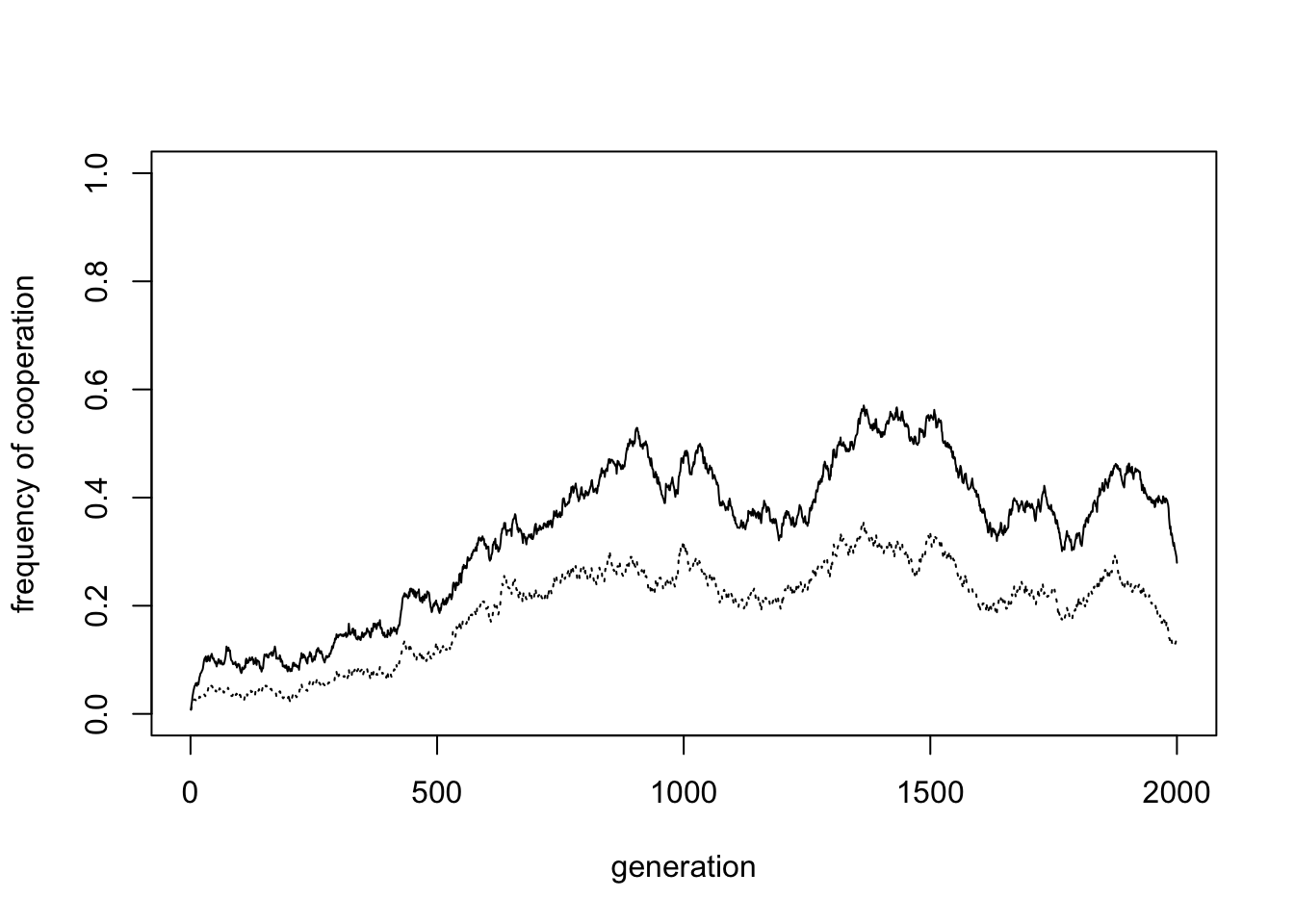
}One run of the model with default values gives the following plot:
In small groups of \(n = 4\), cooperation increases to around 0.8. For the above output, the mean cooperation in the final 50% of timesteps is 0.84. A slight majority are Ps, with the rest Cs.
A look at a sample of the final generation population shows that groups are quite homogenous, comprising either all Ps, all Cs or all Ds. There are some dissimilar agents, most likely due to mutation or between-group social learning. This within-group homogeneity and between-group heterogeneity is a hallmark of cultural group selection.
##      [,1] [,2] [,3] [,4] [,5] [,6] [,7] [,8] [,9] [,10] [,11] [,12] [,13] [,14]
## [1,] "D"  "P"  "P"  "P"  "D"  "P"  "P"  "P"  "P"  "P"   "P"   "C"   "P"   "P"
## [2,] "D"  "P"  "P"  "P"  "P"  "P"  "P"  "P"  "P"  "P"   "P"   "C"   "P"   "P"
## [3,] "D"  "P"  "P"  "P"  "P"  "P"  "P"  "P"  "P"  "P"   "P"   "C"   "P"   "P"
## [4,] "D"  "P"  "P"  "P"  "P"  "P"  "P"  "P"  "P"  "P"   "P"   "C"   "P"   "P"
##      [,15] [,16] [,17] [,18] [,19] [,20] [,21] [,22] [,23] [,24] [,25]
## [1,] "P"   "P"   "D"   "D"   "P"   "D"   "C"   "P"   "C"   "C"   "C"
## [2,] "P"   "P"   "D"   "D"   "P"   "D"   "C"   "P"   "C"   "C"   "C"
## [3,] "P"   "P"   "D"   "C"   "P"   "D"   "C"   "P"   "C"   "C"   "C"
## [4,] "C"   "P"   "D"   "C"   "P"   "D"   "C"   "C"   "C"   "C"   "C"
Increasing the group size to \(n = 32\) reduces the frequency of cooperation slightly, to around 0.7.
In the plot above, the mean cooperation in the last 50% of timesteps is 0.7. It is a well-established finding that cooperation is harder to maintain in larger groups, but here cooperation only slightly declines.
By setting \(p = k = 0\) we can remove punishment from the model:
Without punishment, cooperation almost disappears (in the plot above, the frequency of cooperation is 0.1). This shows that, even with group selection, some mechanism is needed to maintain cooperation within groups. These cooperative groups are then favoured by group selection. But if there is no such mechanism, group selection has nothing to select.
Conversely, we can remove group selection by setting the probability of inter-group competition \(\varepsilon = 0\), and restoring punishment.
Again, cooperation has all but disappeared (to 0.16 in the above plot). Without group selection, cooperation has no benefit, and is selected against.
Now let’s increase the inter-group mixing rate from \(m = 0.01\) to \(m = 0.05\):
Inter-group mixing reduces cooperation (in the plot above to 0.42). Mixing, like migration, breaks down between-group variation and prevents group selection from acting. Because mixing operates alongside payoff-biased social learning, and defectors typically have higher fitness than cooperators, this results in the spread of defectors.
Finally, let’s recreate one of the figures from Boyd et al. (2003). Their Figure 1b shows the frequency of cooperation across a range of group sizes (\(n\)), for three different rates of intergroup conflict (\(\varepsilon\)). The following code recreates this figure. Warning: it can take a while to run so many simulations. (NB Boyd et al. took an average of 10 independent runs for each parameter combination and went up to \(n = 256\); the code below only has one run per parameter combination and goes up to \(n = 64\). However, the results are qualitatively the same.)
n <- c(4,8,16,32,64)
epsilon <- c(0.0075,0.015,0.03)

output <- data.frame(matrix(NA, ncol = length(epsilon), nrow = length(n)))
rownames(output) <- n
colnames(output) <- epsilon

for (j in 1:length(epsilon)) {

  for (i in 1:length(n)) {

    output[i,j] <- Cooperation(n = n[i],
                               epsilon = epsilon[j],
                               show_plot = FALSE)$mean_coop

  }

}

plot(x = 1:length(n), y = output[,1],
     type = 'o',
     ylab = "frequency of cooperation",
     xlab = "group size",
     col = "darkblue",
     pch = 15,
     ylim = c(0,1),
     xlim = c(1,length(n)),
     xaxt = "n")

axis(1, at=1:length(n), labels=n)

lines(x = 1:length(n), output[,2],
      type = 'o',
      col = "red",
      pch = 17)

lines(x = 1:length(n), output[,3],
      type = 'o',
      col = "plum",
      pch = 16)

legend("bottomleft",
        legend = epsilon,
        title = "freq of group conflict",
        lty = 1,
        lwd = 2,
        pch = c(15,17,16),
        col = c("darkblue", "red","plum"),
        bty = "n",
        cex = 0.9)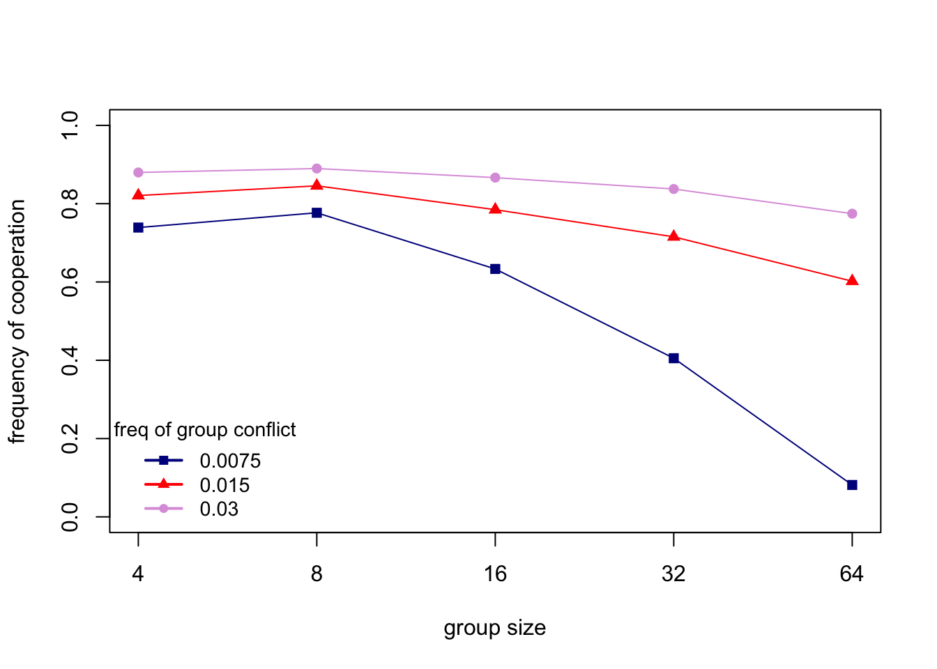
The above figure shows that (i) cooperation declines with group size; (ii) higher rates of inter-group conflict maintain higher frequencies of cooperation; and (iii) at the highest rates of inter-group conflict, cooperation is maintained even in large groups.
Summary
Cooperation underpins the social lives of countless species, including (and perhaps especially) human societies. Given the advantage that free-riders have over cooperators, cooperation requires special explanation. Many such explanations have been offered. Model 11, recreating a model by Boyd et al. (2003), provides one such explanation, combining altruistic punishment, payoff-biased social learning and cultural group selection.
We found, as did Boyd et al. (2003), that cooperation can be maintained in relatively large groups when these processes are acting together. Within groups, payoff-biased social learning is the selection mechanism. Because defectors have higher payoffs than cooperators, defection is selected and spreads within groups. Adding punishers turns the tables, with defectors’ payoffs reduced by punishment. Yet without group selection, altruistic punishers will be out-competed by non-punishing cooperators, who benefit from others’ punishment but do not pay the costs of punishing. But then we are back where we started, and defectors will out-compete the non-punishing cooperators. With group selection, however, groups of cooperating punishers spread at the expense of groups of defectors due to the benefit of cooperation in inter-group competition. Hence, cooperation spreads. Neither punishment nor group selection alone maintain cooperation; both are needed.
The model presented here is one version of a broad class of models of cultural group selection (Smith 2020). This one involves punishment. Others assume that rapid cultural adaptation or conformity maintain between-group cultural variation, and inter-group competition favours more-cooperative groups. Some models assume preferential migration plus acculturation (see Model 7) rather than group extinction/replacement as we simulated here. There is no single ‘cultural group selection’ hypothesis, there are several. It is important to recognise that within-group mechanisms like punishment are not alternatives to cultural group selection, but rather are complementary. In Model 11, punishment favours cooperation within groups, while group selection solves the second-order free-rider problem that comes with punishment.
Cultural group selection is a controversial explanation for human cooperation (see Richerson et al. 2016 and associated commentaries; and also Smith 2020). This may be a legacy of the rejection of naive genetic group selection in biology in the 1960s. However, cultural group selection is different: it involves cultural rather than genetic variation, it applies only to humans, and it incorporates special assumptions about biased social learning, inter-group interactions etc. Nevertheless, models like Model 11 are just that: models. Evidence is needed to demonstrate that cultural group selection has been an important driver of cooperation in real human societies. Some such evidence exists, such as findings of substantial between-group cultural variation in cooperation-related behaviours (Richerson et al. 2016). Other evidence opposes cultural group selection, such as findings that people do not reliably socially learn cooperative behaviour (Lamba 2014). The value of models like Model 11 lies in clarifying theoretical assumptions and predictions, allowing those assumptions and predictions to be tested empirically.
In terms of programming, Model 11 is probably the most complex in this series so far. There are several stages within each timestep, and more parameters than any previous model. As a result, run times can be slow, particularly for large groups. Where possible we used matrices rather than dataframes and vectorised the code to improve speed. Unfortunately there is no straightforward way of vectorising the punishment and social learning stages (if you can think of one let me know!). We must accept that sometimes complex models take a while to run. Grab a cup of tea and watch TV, smug in the knowledge that your code is working for you in the background. More seriously, the important thing with complex models is to make and test each stage in turn under manageable assumptions (e.g. \(N = 4\) rather than \(N = 128\)) before putting them all together, as we did above. This makes it much easier to catch bugs and to make sure that your code does what you think it does.
Exercises
Use the Cooperation function to explore the effect of the remaining parameters on the frequency of cooperation: (a) the error rate \(e\); (b) the cost of cooperation \(c\); (c) the mutation rate \(\mu\); and (d) the number of groups \(N\).
Recreate Boyd et al.’s (2003) other figures, adapting the code above used to recreate their Figure 1b. Do you get the same results?
Change the starting conditions, to (a) one group of all Cs and the rest all Ds; (b) all Ds (with Ps and Cs only appearing via mutation); and (c) random behaviours. Does cooperation still emerge with these different starting conditions?
Add a new parameter \(b\) to the Cooperation function. Each cooperator (Cs and Ps with probability \(1 - e\)) generates a payoff benefit \(b\) which is shared equally amongst all group members (including defectors). This simulates the standard ‘Public Goods Game’ from economics. Now cooperation generates within-group benefits, as well as between-group benefits via group selection. Explore the effect of different values of \(b\) on overall cooperation levels.
References
Apicella, C. L., & Silk, J. B. (2019). The evolution of human cooperation. Current Biology, 29(11), R447-R450.
Boyd, R., Gintis, H., Bowles, S., & Richerson, P. J. (2003). The evolution of altruistic punishment. Proceedings of the National Academy of Sciences, 100(6), 3531-3535.
Lamba, S. (2014). Social learning in cooperative dilemmas. Proceedings of the Royal Society B, 281(1787), 20140417.
Richerson, P., Baldini, R., Bell, A. V., Demps, K., Frost, K., Hillis, V., … & Zefferman, M. (2016). Cultural group selection plays an essential role in explaining human cooperation: A sketch of the evidence. Behavioral and Brain Sciences, 39, E30.
Smith, D. (2020). Cultural group selection and human cooperation: a conceptual and empirical review. Evolutionary Human Sciences, 2.
West, S. A., Griffin, A. S., & Gardner, A. (2007). Evolutionary explanations for cooperation. Current Biology, 17(16), R661-R672.