Model 4: Biased transmission (indirect bias)
Introduction
In Model 3 we examined direct bias, where certain cultural traits are preferentially copied from a randomly chosen demonstrator. Here we will simulate indirect bias (Boyd & Richerson 1985). This is another form of biased transmission, or cultural selection, but where certain demonstrators are more likely to be copied than other demonstrators. For this reason, indirect bias is sometimes called ‘demonstrator-based’ or ‘context’ bias.
Indirect bias comes in several forms. Learners might preferentially copy demonstrators who have high success or payoffs (which may or may not derive from their cultural traits), demonstrators who are old (and perhaps have accrued valuable knowledge, or at least good enough to keep them alive to old age), demonstrators who are the same gender as the learner (if cultural traits are gender-specific), or demonstrators who possess high social status or prestige.
Model 4 presents a simple model of indirect bias, first showing how payoff-based indirect bias can look very similar to payoff-based direct bias (Model 4a), then exploring a more interesting case when payoff-based indirect bias allows a neutral trait to ‘hitch-hike’ along with a high-payoff functional trait when both are exhibited by high payoff demonstrators (Model 4b).
Model 4a: Payoff bias
In Model 4a we will simulate a case where new agents preferentially copy the cultural traits of agents from the previous generation who have higher relative payoffs. This is sometimes called ‘payoff’ or ‘success’ bias.
We will start with the skeleton of Model 3. As in Model 3, there are \(N\) agents, each of whom possess a single cultural trait, either \(A\) or \(B\). The frequency of trait \(A\) is denoted \(p\), and the initial frequency in the first generation is \(p_0\). There are \(t_{max}\) timesteps and \(r_{max}\) independent runs.
In Model 3, agents were picked at random from the previous generation, and if that randomly-chosen agent possessed trait \(A\) then trait \(A\) was copied with probability \(s\). For indirect bias, we need to change this. Demonstrator choice is no longer random: demonstrators are chosen non-randomly based on their payoffs. To implement this, we need to specify payoffs for each agent.
We will assume that an agent’s payoff is determined solely by the agent’s cultural trait. Agents with trait \(B\) have payoff of \(1\) (a ‘baseline’ payoff), while agents with trait \(A\) have payoff of \(1 + s\). This means that trait \(A\) gives a payoff advantage to its bearers, relative to agents possessing trait \(B\). The larger is \(s\), the bigger this relative advantage.
Payoff-based indirect bias is then implemented by making the probability that an agent is chosen as a demonstrator proportional to that agents’ relative payoff, i.e. its payoff relative to all other agents in the population. Once an agent is chosen, its trait is copied with no error and with probability 1.
Rather than going straight to a simulation function, let’s explore this notion of relative payoff a bit further. First let’s create a population of \(N\) agents, with traits determined by \(p_0\), as usual.
N <- 1000
p_0 <- 0.5
s <- 0.1

agent <- data.frame(trait = sample(c("A","B"), N, replace = TRUE,
                    prob = c(p_0,1-p_0)))

head(agent)
## trait
## 1 B
## 2 B
## 3 A
## 4 B
## 5 A
## 6 BGiven that \(p_0 = 0.5\), you should see that the first few agents have a mix of trait \(A\) and trait \(B\). Now let’s add a payoff variable to the agent dataframe:
##   trait payoff
## 1     B    1.0
## 2     B    1.0
## 3     A    1.1
## 4     B    1.0
## 5     A    1.1
## 6     B    1.0
Agents with trait \(A\) are given fitness \(1 + s\), which in this case is 1.1, while agents with trait \(B\) are given fitness of 1.
The relative payoff of an agent can be calculated by dividing its payoff by the sum of all payoffs of all agents:
## [1] 0.0009526531 0.0009526531 0.0010479185 0.0009526531 0.0010479185
## [6] 0.0009526531## [1] 1These relative payoffs are obviously much smaller than the absolute payoffs because they have all been divided by \(N\), which is a large number. They also all add up to 1. This is useful because in our simulation we can set the probability of picking an agent from whom to copy as equal to its relative fitness. Probabilities, like our relative payoffs, must sum to 1.
In previous models we implemented random copying by using the sample command to pick \(N\) previous-generation agents at random to copy. This worked because by default the sample command picks each item - in our case, each previous-generation agent - with equal probability. However, we can override this default by adding a prob argument. If we set prob to be our relative_payoffs, then each agent will be chosen in proportion to its relative payoff. The following code does this for one new generation, after putting agent into previous_agent.
previous_agent <- agent

agent$trait <- sample(previous_agent$trait, N, replace = TRUE, prob = relative_payoffs)

sum(previous_agent$trait == "A") / N
## [1] 0.497## [1] 0.491You should see that the frequency of trait \(A\) has increased from previous_agent to our new agent generation. This is what we would expect, given that there is a greater chance of selecting agents with the higher payoff trait \(A\).
The following function incorporates the preceding code into our standard simulation model:
IndirectBias <- function (N, s, p_0, t_max, r_max) {

  # create a matrix with t_max rows and r_max columns, fill with NAs, convert to dataframe
  output <- as.data.frame(matrix(NA, t_max, r_max))

  # purely cosmetic: rename the columns with run1, run2 etc.
  names(output) <- paste("run", 1:r_max, sep="")

  for (r in 1:r_max) {

    # create first generation
    agent <- data.frame(trait = sample(c("A","B"), N, replace = TRUE,
                        prob = c(p_0,1-p_0)))

    # add payoffs
    agent$payoff[agent$trait == "A"] <- 1 + s
    agent$payoff[agent$trait == "B"] <- 1

    # add first generation's p to first row of column r
    output[1,r] <- sum(agent$trait == "A") / N

    for (t in 2:t_max) {

      # copy agent to previous_agent dataframe
      previous_agent <- agent

      # get relative payoffs of previous agents
      relative_payoffs <- previous_agent$payoff / sum(previous_agent$payoff)

      # new traits copied from previous generation, biased by payoffs
      agent$trait <- sample(previous_agent$trait,
                            N, replace = TRUE,
                            prob = relative_payoffs)

      # add payoffs
      agent$payoff[agent$trait == "A"] <- 1 + s
      agent$payoff[agent$trait == "B"] <- 1

      # get p and put it into output slot for this generation t and run r
      output[t,r] <- sum(agent$trait == "A") / N

    }

  }

  # first plot a thick line for the mean p
  plot(rowMeans(output),
       type = 'l',
       ylab = "p, proportion of agents with trait A",
       xlab = "generation",
       ylim = c(0,1),
       lwd = 3,
       main = paste("N = ", N, ", s = ", s, sep = ""))

  for (r in 1:r_max) {

    # add lines for each run, up to r_max
    lines(output[,r], type = 'l')

  }

  output  # export data from function
}
Now we can run IndirectBias with a small payoff advantage to agents with trait \(A\):
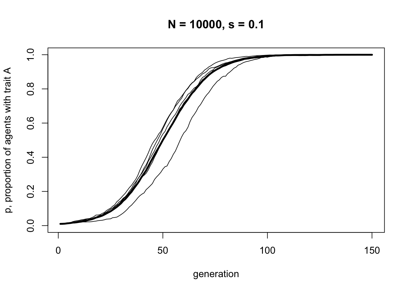
This S-shaped curve is very similar to the one we generated in Model 3 for direct bias, with the same value of \(s = 0.1\). This is not too surprising, given that in Model 4a an agent’s payoff is entirely determined by their cultural trait. Under these assumptions, preferentially copying high payoff agents is functionally equivalent to preferentially copying high payoff traits. This is not always the case, however, as we will see in Model 4b.
Model 4b: Cultural hitch-hiking
A more interesting case of indirect bias occurs when individuals possess two cultural traits, one functional and the other neutral. Under certain circumstances, payoff based indirect bias can cause the neutral trait to ‘hitch-hike’ alongside the functional trait. Neutral traits can spread in the population simply because they are associated with high payoff traits in high payoff demonstrators, even though they have no effect on payoffs themselves.
The trait already incorporated into IndirectBias above is functional, in that one of its variants, \(A\), has higher payoff than the alternative variant, \(B\), when \(s > 0\) (or vice versa when \(s < 0\)). A neutral trait has no effect on payoffs, and all variants are equally effective, much like the trait subject to unbiased transmission in Model 1.
In Model 4b we will add a neutral trait to IndirectBias. We keep the functional trait 1 that can be either \(A\) or \(B\), with payoff advantage \(s\) to trait \(A\). We add a second trait, trait 2, which can be either \(X\) or \(Y\). We define \(q\) as the proportion of \(X\) in trait 2, with \(1 - q\) the proportion of \(Y\). Whether an individual has trait \(X\) or \(Y\) has no effect on their payoff.
We will model a situation where the two traits may be initially linked. We are not going to be concerned here with why the two traits are initially linked. The link could, for example, have arisen by chance due to drift in historically small populations. We will leave this as an assumption of our model, which is fine as long as we are explicit about this. We define a parameter \(L\) that specifies the probability in the initial generation (at \(t = 1\)) that, if an individual has an \(A\) for trait 1, they also have an \(X\) for trait 2. With probability \(1 - L\), they pick \(X\) with probability \(q_0\), analogously to how \(p_0\) specifies the probability of picking an \(A\) for trait 1 in the first generation). In this model, \(q_0\) will be fixed at 0.5, i.e. an equal chance of having \(X\) or \(Y\).
The following code defines a new agent dataframe. What was previously trait now becomes trait1. A new trait2 is initially set to NA for all agents. We then, with probability \(L\), link trait2 to trait1, otherwise set trait2 at random.
N <- 1000
p_0 <- 0.5
q_0 <- 0.5
L <- 1

agent <- data.frame(trait1 = sample(c("A","B"), N, replace = TRUE,
                                    prob = c(p_0,1-p_0)),
                    trait2 = rep(NA, N))

# with prob L, trait 2 is tied to trait 1, otherwise trait X with prob q_0
prob <- runif(N)
agent$trait2[agent$trait1 == "A" & prob < L] <- "X"
agent$trait2[agent$trait1 == "B" & prob < L] <- "Y"

agent$trait2[prob >= L] <- sample(c("X","Y"), sum(prob >= L), replace = TRUE,
                                  prob = c(q_0,1-q_0))

head(agent)
## trait1 trait2
## 1 A X
## 2 A X
## 3 B Y
## 4 A X
## 5 A X
## 6 A XWhen \(L=1\), there is maximum linkage between the two traits. All individuals with \(A\) also have \(X\), and all individuals with \(B\) have \(Y\). As \(L\) gets smaller, this linkage breaks down.
Now we can insert this code into the IndirectBias function from above, with a few other additions. Note that payoffs are calculated exactly as before, based solely on whether trait1 is \(A\) or \(B\). The demonstrators are picked as before, based on relative_payoffs, except now trait2 is copied from the same demonstrator alongside trait1. Finally, we create an additional output dataframe for trait2, use this second output dataframe to record \(q\), the frequency of \(X\) in trait 2, in each timestep, and use it to plot both \(p\) and \(q\) in different colours. Note the new legend command, which allows us to label the two lines in the plot, and the use of list to export two output dataframes, rather than one.
IndirectBias2 <- function (N, s, L, p_0, q_0, t_max, r_max) {

  # create matrices with t_max rows and r_max columns, fill with NAs, convert to dataframe
  output_trait1 <- as.data.frame(matrix(NA, t_max, r_max))
  output_trait2 <- as.data.frame(matrix(NA, t_max, r_max))

  # purely cosmetic: rename the columns with run1, run2 etc.
  names(output_trait1) <- paste("run", 1:r_max, sep="")
  names(output_trait2) <- paste("run", 1:r_max, sep="")

  for (r in 1:r_max) {

    # create first generation
    agent <- data.frame(trait1 = sample(c("A","B"), N, replace = TRUE,
                                        prob = c(p_0,1-p_0)),
                        trait2 = rep(NA, N))

    # with prob L, trait 2 is tied to trait 1, otherwise trait X with prob q_0
    prob <- runif(N)
    agent$trait2[agent$trait1 == "A" & prob < L] <- "X"
    agent$trait2[agent$trait1 == "B" & prob < L] <- "Y"

    agent$trait2[prob >= L] <- sample(c("X","Y"), sum(prob >= L), replace = TRUE,
                                      prob = c(q_0,1-q_0))

    # add payoffs
    agent$payoff[agent$trait1 == "A"] <- 1 + s
    agent$payoff[agent$trait1 == "B"] <- 1

    # add first generation's p and q to first row of column r
    output_trait1[1,r] <- sum(agent$trait1 == "A") / N
    output_trait2[1,r] <- sum(agent$trait2 == "X") / N

    for (t in 2:t_max) {

      # copy agent to previous_agent dataframe
      previous_agent <- agent

      # get relative payoffs of previous agents
      relative_payoffs <- previous_agent$payoff / sum(previous_agent$payoff)

      # new traits copied from previous generation, biased by payoffs
      demonstrators <- sample(1:N,
                              N, replace = TRUE,
                              prob = relative_payoffs)

      agent$trait1 <- previous_agent$trait1[demonstrators]
      agent$trait2 <- previous_agent$trait2[demonstrators]

      # add payoffs
      agent$payoff[agent$trait1 == "A"] <- 1 + s
      agent$payoff[agent$trait1 == "B"] <- 1

      # put p and q into output slot for this generation t and run r
      output_trait1[t,r] <- sum(agent$trait1 == "A") / N
      output_trait2[t,r] <- sum(agent$trait2 == "X") / N

    }

  }

  # first plot a thick grey line for the mean p
  plot(rowMeans(output_trait1),
       type = 'l',
       ylab = "proportion of agents with trait A (orange) or X (blue)",
       xlab = "generation",
       ylim = c(0,1),
       lwd = 3,
       main = paste("N = ", N, ", s = ", s, ", L = ", L, sep = ""),
       col = "orange")

  # now thick orange line for mean q
  lines(rowMeans(output_trait2), col = "royalblue", lwd = 3)

  for (r in 1:r_max) {

    # add lines for each run, up to r_max
    lines(output_trait1[,r], type = 'l', col = "orange")
    lines(output_trait2[,r], type = 'l', col = "royalblue")

  }

  legend("bottomright",
         legend = c("p (trait 1)", "q (trait 2)"),
         lty = 1,
         lwd = 3,
         col = c("orange", "royalblue"),
         bty = "n")

  list(output_trait1, output_trait2)  # export data from function

  }
Now we can run IndirectBias2 with a high linkage between trait 1 and trait 2, \(L = 0.9\)
data_model4b <- IndirectBias2(N = 10000,
                              s = 0.1,
                              L = 0.9,
                              p_0 = 0.01,
                              q_0 = 0.5,
                              t_max = 150,
                              r_max = 5)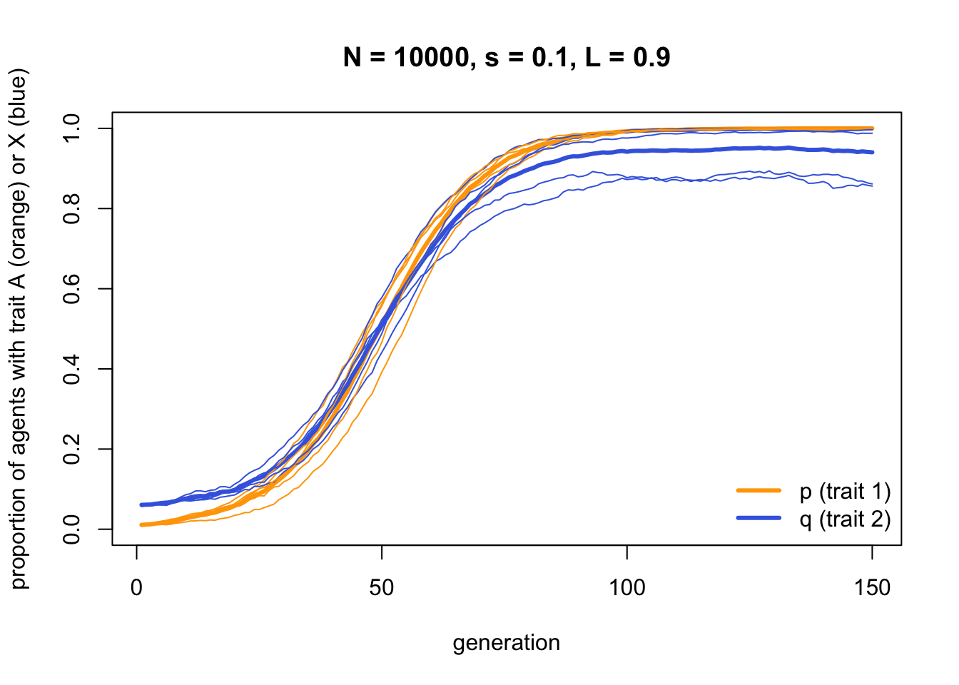
As you might expect, trait \(A\) (the orange line) goes to fixation exactly as for IndirectBias above. However, trait \(X\) (the blue line) shows a similar increase - not quite all the way to fixation, because \(L < 1\), but very nearly. Hence the neutral trait \(X\) is hitch-hiking along with the functional trait \(A\) due to payoff based indirect bias. Trait \(X\) has no effect on payoffs, but because it happens to be associated with trait \(A\) at the start, it spreads through the population.
If we remove the linkage by setting \(L = 0\), we see that this hitch-hiking no longer occurs. Instead trait \(X\) drifts randomly as we would expect for a neutral trait:
data_model4b <- IndirectBias2(N = 10000,
                              s = 0.1,
                              L = 0.0,
                              p_0 = 0.01,
                              q_0 = 0.5,
                              t_max = 150,
                              r_max = 5)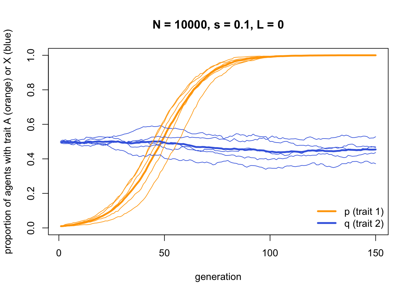
And when we remove the payoff biased indirect bias by setting \(s = 0\), and reintroduce the linkage (\(L = 0.9\)), neither trait increases in frequency. Both are now effectively neutral.
data_model4b <- IndirectBias2(N = 10000,
                              s = 0.0,
                              L = 0.9,
                              p_0 = 0.3,
                              q_0 = 0.5,
                              t_max = 150,
                              r_max = 5)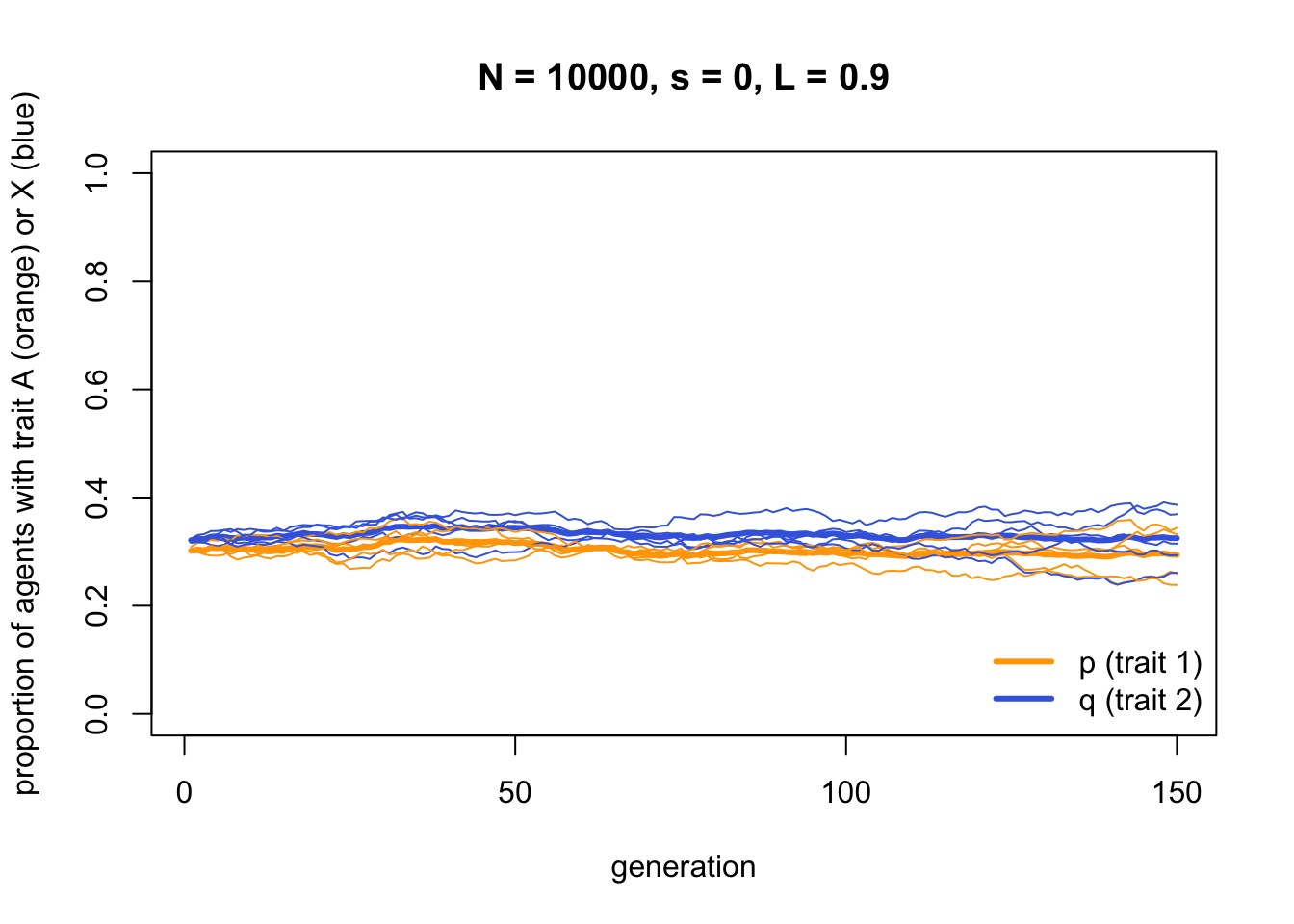
Summary
Indirect bias occurs when individuals preferentially learn from demonstrators who have particular characteristics, such as being wealthy or socially successful (having high ‘payoffs’ in the language of modelling), being old, having a particular gender, or being prestigious. There is extensive evidence for these indirect transmission biases from the broad social and behavioural sciences (e.g. Rogers 2010; Labov 1972; Bandura, Ross & Ross 1963) and cultural evolution research specifically (e.g. Mesoudi 2011; Henrich & Gil-White 2001; Brand et al. 2020; Wood et al. 2012; McElreath et al. 2008; Henrich & Henrich 2010). Consequently, it is worth modelling indirect bias to understand its dynamics, and how it is similar or different to other forms of biased transmission.
Our first simple model of indirect bias, Model 4a, showed that when individuals preferentially learn from high payoff demonstrators, and demonstrator payoff is determined directly by the demonstrator’s cultural trait, then the trait that gives demonstrators higher relative payoff spreads through the population. This is entirely expected and intuitive. The resulting S-shaped diffusion curve for Model 4a looks extremely similar to that generated in Model 3 for direct bias with the same selection parameter \(s\). This is to be expected, given our assumptions that demonstrator payoff is determined solely by trait payoff. So in this case direct bias and indirect bias are functionally equivalent.
This should strike a note of caution. If we see the same cultural dynamics generated from different underlying models, then we cannot be certain which of these underlying processes generated similar real-world cultural dynamics. Nevertheless, it’s better to know this, than to incorrectly attribute a dynamic to the wrong process.
Model 4b examined the more interesting case where there are two cultural traits, one functional and one neutral. If these traits are initially linked, via our parameter \(L\), then the neutral trait can hitch-hike along with the functional trait. Everyday examples of cultural hitch-hiking might be where people copy fashion styles from wealthy and talented sportstars: a footballer’s tattoos or hairstyle is unlikely to have anything to do with their sporting success, but these neutral traits may nevertheless be copied if people generally copy all traits associated with successful demonstrators. There is experimental evidence for cultural hitch-hiking (Mesoudi & O’Brien 2008), while Yeh et al. (2019) have created more elaborate models of cultural hitch-hiking with more than two traits and copyable links between those traits.
While we did not model the evolution of indirect bias itself, we might imagine that this global copying of successful demonstrators might be less costly to the learner when demonstrators exhibit multiple traits than direct bias, where learners would have to identify which of the multiple traits actually contribute to the demonstrator’s success. The cost of indirect bias is potentially copying neutral traits, as we saw in Model 4b, or even maladaptive traits, alongside the functional traits. But in some circumstances this cost may be less than the aforementioned cost of direct bias. If it is, then this may be an explanation for the presence of neutral or maladaptive traits in human culture.
Boyd & Richerson (1985) modelled another interesting case of indirect bias, where the criterion of demonstrator success is copied alongside the actual cultural trait. For example, one might copy not only the specific tattoo of a successful footballer, but also copy their preference for tattoos. Under certain conditions this can lead to the runaway selection of both traits and preferences, with both getting more and more extreme over time. In our example this would lead to more and more extensive tattoos (which perhaps has happened in Micronesia, but for yam-growing rather than football: Boyd & Richerson 1985). This is roughly analogous to runaway sexual selection in genetic evolution that can lead to elaborate traits such as peacock’s tails, which may occur because both elaborate tails and preferences for elaborate tails are genetically inherited together. Both cultural hitch-hiking and runaway selection are interesting dynamics of indirectly bias which are not observed for direct bias.
In terms of programming innovations, we saw in Model 4a how to assign payoffs to different agents on the basis of their cultural trait, and then use the relative_payoffs in the sample command to implement payoff-based selection of demonstrators from whom to learn. In Model 4b we introduced a second trait, keeping track of both the frequency of \(A\) in trait 1 (\(p\)) and the frequency of \(X\) in trait 2 (\(q\)). We also saw how to link these traits together using the \(L\) parameter. Finally, we saw how to draw two results lines on the same plot in different colours, include a legend for those lines, and export multiple dataframes from the simulation function as a list.
Exercises
Try different values of \(s\) in IndirectBias to confirm that larger \(s\) increases the speed with which \(A\) goes to fixation.
Try different values of \(L\) in IndirectBias2 to confirm that as \(L\) gets smaller, the hitch-hiking effect gets weaker.
In IndirectBias2 the hitch-hiking trait is neutral. But can a detrimental trait also hitch-hike? Modify the function to make the second trait functional, with a payoff disadvantage to \(X\) over \(Y\) (e.g. by introducing an equivalent selection parameter to \(s\) which affects \(X\) relative to \(Y\), and making this new parameter negative). Set the initial linkage conditions such that the high payoff trait1 variant \(A\) is associated with the low payoff trait2 variant \(X\). Are there any conditions under which the detrimental, low-payoff trait \(X\) hitch-hikes on the beneficial, high-payoff trait \(A\)?
Analytical Appendix
In Model 4a, the frequency of trait \(A\) in the next generation, \(p'\), is simply the relative payoff of all agents with trait \(A\) in the previous generation. This is given by:
\[p' = \frac{p(1+s)}{ p(1+s) + (1-p)} = \frac{p(1+s)}{ 1 + sp} \hspace{30 mm}(4.1)\]
where \(p(1+s)\) is the payoff of all agents with trait \(A\), and \((1-p)\) is the payoff of all agents with trait \(B\).
Plotting this recursion gives a curve that matches the one generated above by the simulation model:
p <- rep(0, 150)
p[1] <- 0.01
s <- 0.1

for (i in 2:150) {
  p[i] <- (p[i-1])*(1+s) / (1 + (p[i-1])*s)
}

plot(p,
     type = 'l',
     ylab = "p, proportion of agents with trait A",
     xlab = "generation",
     ylim = c(0,1),
     lwd = 3,
     main = paste("s = ", s, sep = ""))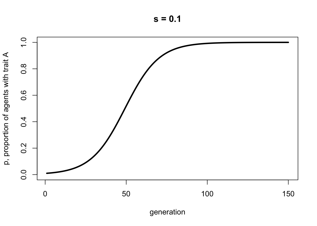
To find the equilibria, we can set \(p'=p\) in Equation 4.1, and rearrange to give:
\[p(1-p)s = 0 \hspace{30 mm}(4.2)\]
This is identical to Equation 3.2, the equivalent for direct bias. Again, there are three equilibria, one when \(p=0\), one when \(s=0\), and one when \(1-p=0\), or when \(p=1\). While Equation 4.1 is not the same as Equation 3.1, the resulting equilibria are identical.
References
Bandura, A., Ross, D., & Ross, S. A. (1963). A comparative test of the status envy, social power, and secondary reinforcement theories of identificatory learning. The Journal of Abnormal and Social Psychology, 67(6), 527.
Boyd, R., & Richerson, P. J. (1985). Culture and the evolutionary process. University of Chicago Press.
Brand, C. O., Heap, S., Morgan, T. J. H., & Mesoudi, A. (2020). The emergence and adaptive use of prestige in an online social learning task. Scientific Reports, 10(1), 1-11.
Henrich, J., & Gil-White, F. J. (2001). The evolution of prestige: Freely conferred deference as a mechanism for enhancing the benefits of cultural transmission. Evolution and Human Behavior, 22(3), 165-196.
Henrich, J., & Henrich, N. (2010). The evolution of cultural adaptations: Fijian food taboos protect against dangerous marine toxins. Proceedings of the Royal Society B: Biological Sciences, 277(1701), 3715-3724.
Labov, W. (1972). Sociolinguistic patterns. University of Pennsylvania press.
McElreath, R., Bell, A. V., Efferson, C., Lubell, M., Richerson, P. J., & Waring, T. (2008). Beyond existence and aiming outside the laboratory: estimating frequency-dependent and pay-off-biased social learning strategies. Philosophical Transactions of the Royal Society B: Biological Sciences, 363(1509), 3515-3528.
Mesoudi, A. (2011). An experimental comparison of human social learning strategies: payoff-biased social learning is adaptive but underused. Evolution and Human Behavior, 32(5), 334-342.
Mesoudi, A., & O’Brien, M. J. (2008). The cultural transmission of Great Basin projectile-point technology I: an experimental simulation. American Antiquity, 73(1), 3-28.
Rogers, E. M. (2010). Diffusion of innovations. Simon and Schuster.
Wood, L. A., Kendal, R. L., & Flynn, E. G. (2012). Context-dependent model-based biases in cultural transmission: Children’s imitation is affected by model age over model knowledge state. Evolution and Human Behavior, 33(4), 387-394.
Yeh, D. J., Fogarty, L., & Kandler, A. (2019). Cultural linkage: the influence of package transmission on cultural dynamics. Proceedings of the Royal Society B, 286(1916), 20191951.