Misc. Analyses

Stratified Analyses

By Sex

Total number of weight samples, by sex, for the 2016 cohort

weight.ls[[2]] %>%
  janitor::tabyl(Gender) %>%
  arrange(desc(n)) %>%
  adorn_pct_formatting() %>%
  tableStyle()

Gender	n	percent
M	1097469	93.3%
F	78526	6.7%

Total number of people

weight.ls[[2]] %>%
  distinct(PatientICN, Gender) %>%
  tabyl(Gender) %>%
  adorn_pct_formatting() %>%
  tableStyle()

Gender	n	percent
F	6200	6.3%
M	92758	93.7%

Association between number of weight samples collected, and Sex/Gender, for the 2016 cohort,

weight.ls[[2]] %>%
  group_by(Gender) %>%
  count(PatientICN) %>%
  summarise(
    mean   = mean(n),
    SD     = sd(n),
    median = median(n),
    min    = min(n),
    max    = max(n)
  ) %>%
  tableStyle()

Gender	mean	SD	median	min	max
F	12.67	12.61	9	1	277
M	11.83	19.05	8	1	1525

Men have, on average, slightly fewer weight values recorded than women in our sample.

Removing the major outlier,

weight.ls[[2]] %>%
  group_by(Gender) %>%
  count(PatientICN) %>%
  filter(n < 1000) %>%
  ggplot(aes(x = Gender, y = n)) %>%
  add(geom_boxplot(fill = "maroon")) %>%
  add(theme_fivethirtyeight(16)) %>%
  add(theme(axis.title = element_text())) %>%
  add(coord_flip()) %>%
  add(labs(
    x = "Sex",
    y = "N Collected Weight Samples"
  ))

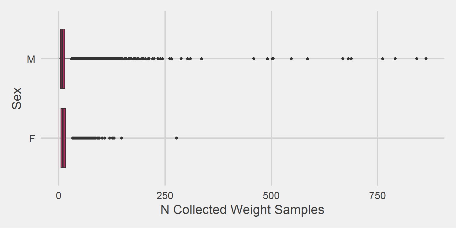
The distribution of outliers differs as well.

All weight in lbs. by sex, for the 2016 cohort only

weight.ls[[2]] %>%
  group_by(Gender) %>%
  summarise(
    mean   = mean(Weight),
    SD     = sd(Weight),
    median = median(Weight),
    min    = min(Weight),
    max    = max(Weight)
  ) %>%
  tableStyle()

Gender	mean	SD	median	min	max
F	184.66	44.56	180.7	0	1479.9
M	209.48	48.45	204.0	0	1486.2

Both Males and Females have implausible maximum weight values.

weight.ls[[2]] %>%
  ggplot(aes(x = Gender, y = Weight)) %>%
  add(geom_boxplot(fill = "maroon")) %>%
  add(theme_fivethirtyeight(16)) %>%
  add(theme(axis.title = element_text())) %>%
  add(coord_flip())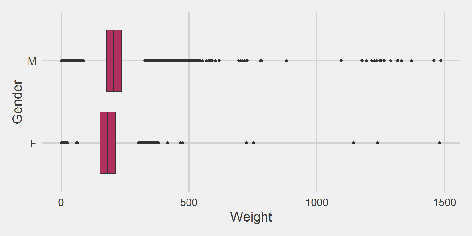

By Algorithm

raw <- weight.ls[[2]] %>%
  select(PatientICN, Weight, Gender)

#---- apply Janney et al. 2016 ----#

Janney2016.df <- Janney2016.f(
  DF = weight.ls[[2]],
  id = "PatientICN",
  measures = "Weight",
  tmeasures = "WeightDateTime",
  startPoint = "VisitDateTime"
) %>%
  select(PatientICN, Weight_OR, Gender) %>%
  rename(Weight = Weight_OR) %>%
  na.omit()

#---- apply Littman et al. 2012 ----#

Littman2012.df <- Littman2012.f(
  DF = weight.ls[[2]],
  id = "PatientICN",
  measures = "Weight",
  tmeasures = "WeightDateTime"
) %>%
  select(PatientICN, OutputMeasurement, Gender) %>%
  rename(Weight = OutputMeasurement) %>%
  na.omit()

#---- Coerce Maciejewski et al. 2016 to a workable format ----#

Maciejewski2016.df <- maciejewski %>%
  filter(IO == "Output", SampleYear == "2016") %>%
  mutate(PatientICN = as.character(PatientICN)) %>%
  left_join(
    raw %>%
      distinct(PatientICN, Gender),
    by = "PatientICN"
  ) %>%
  select(PatientICN, Weight, Gender) %>%
  na.omit()

#---- Apply Breland et al. 2017 ----#

Breland2017.df <- Breland2017.f(
  DF = weight.ls[[2]],
  id = "PatientICN",
  measures = "Weight",
  tmeasures = "WeightDateTime"
) %>%
  select(PatientICN, measures_aug_, Gender) %>%
  rename(Weight = measures_aug_) %>%
  na.omit()

#---- Apply Maguen et al. 2013 ----#

Maguen2013.df <- Maguen2013.f(
  DF = weight.ls[[2]],
  id = "PatientICN",
  measures = "Weight",
  tmeasures = "WeightDateTime",
  variables = c("AgeAtVisit", "Gender")
) %>%
  select(PatientICN, Output, Gender) %>%
  rename(Weight = Output) %>%
  na.omit()

#---- Apply Goodrich 2016 ----#

Goodrich2016.df <- Goodrich2016.f(
  DF = weight.ls[[2]],
  id = "PatientICN",
  measures = "Weight",
  tmeasures = "WeightDateTime",
  startPoint = "VisitDateTime"
) %>%
  select(PatientICN, output, Gender) %>%
  rename(Weight = output) %>%
  na.omit()

#---- Apply Chan & Raffa 2017 ----#

Chan2017.df <- Chan2017.f(
  DF = weight.ls[[2]],
  id = "PatientICN",
  measures = "Weight",
  tmeasures = "WeightDateTime"
) %>%
  select(PatientICN, measures_aug_, Gender) %>%
  rename(Weight = measures_aug_) %>%
  na.omit()

#---- Apply Jackson et al. 2015 ----#

Jackson2015.df <- Jackson2015.f(
  DF = weight.ls[[2]],
  id = "PatientICN",
  measures = "Weight",
  tmeasures = "WeightDateTime",
  startPoint = "VisitDateTime"
) %>%
  left_join(
    weight.ls[[2]] %>%
      distinct(PatientICN, Gender),
    by = "PatientICN"
  ) %>%
  select(PatientICN, Gender, output) %>%
  rename(Weight = output) %>%
  na.omit()

#---- Apply Buta et al., 2018 ----#

Buta2018.df <- Buta2018.f(
  DF = weight.ls[[2]],
  id = "PatientICN",
  measures = "BMI",
  tmeasures = "WeightDateTime"
) %>%
  select(PatientICN, Gender, Weight) %>%
  na.omit()

#---- Apply Kazerooni & Lim, 2016 ----#

Kazerooni2016.df <- Kazerooni2016.f(
  DF = weight.ls[[2]],
  id = "PatientICN",
  measures = "Weight",
  tmeasures = "WeightDateTime",
  startPoint = "VisitDateTime"
) %>%
  select(PatientICN, Gender, Weight) %>%
  na.omit()

#---- Apply Noel et al., 2012 ----#

Noel2012.df <- Noel2012.f(
  DF = weight.ls[[2]],
  id = "PatientICN",
  measures = "Weight",
  tmeasures = "WeightDateTime"
) %>% 
  distinct(PatientICN, Gender, FYQ, Qmedian) %>%
  select(-FYQ) %>%
  rename(Weight = Qmedian) %>%
  na.omit()

#---- Apply Rosenberger et al., 2011 ----#

Rosenberger2011.df <- Rosenberger2011.f(
  DF = weight.ls[[2]],
  id = "PatientICN",
  tmeasures = "WeightDateTime",
  startPoint = "VisitDateTime",
  pad = 1
) %>%
  select(PatientICN, Gender, Weight) %>%
  na.omit()

# stack original (raw), janney 2016, littman 2012, maciejewski 2016, 
# Breland 2017, Maguen 2013, Goodrich 2016, Chan & Raffa 2017, 
# Jackson 2015, Buta 2018, Kazerooni & Lim 2016, Noel 2012,
# and Rosenberger 2011 processed weights
  
algos.fac  <- c("Raw Weights",
                "Janney 2016",
                "Littman 2012",
                "Maciejewski 2016",
                "Breland 2017",
                "Maguen 2013",
                "Goodrich 2016",
                "Chan 2017",
                "Jackson 2015",
                "Buta 2018",
                "Kazerooni 2016",
                "Noel 2012",
                "Rosenberger 2011")

DF <- bind_rows(
  list(`Raw Weights`      = raw,
       `Janney 2016`      = Janney2016.df,
       `Littman 2012`     = Littman2012.df,
       `Maciejewski 2016` = Maciejewski2016.df,
       `Breland 2017`     = Breland2017.df,
       `Maguen 2013`      = Maguen2013.df,
       `Goodrich 2016`    = Goodrich2016.df,
       `Chan 2017`        = Chan2017.df,
       `Jackson 2015`     = Jackson2015.df,
       `Buta 2018`        = Buta2018.df,
       `Kazerooni 2016`   = Kazerooni2016.df,
       `Noel 2012`        = Noel2012.df,
       `Rosenberger 2011` = Rosenberger2011.df),
  .id = "Algorithm"
)

rm(
  Buta2018.df,
  Kazerooni2016.df,
  Noel2012.df,
  Rosenberger2011.df,
  Breland2017.df,
  Chan2017.df,
  Goodrich2016.df,
  Jackson2015.df,
  Janney2016.df,
  Littman2012.df,
  Maciejewski2016.df,
  Maguen2013.df,
  raw
)

DF$Algorithm <- factor(DF$Algorithm, levels = algos.fac, labels = algos.fac)

DF$Type <- case_when(
  DF$Algorithm == "Raw Weights"                  ~ 1,
  DF$Algorithm %in% algos.fac[c(2, 7, 9, 11:13)] ~ 2,
  DF$Algorithm %in% algos.fac[c(3:6, 8, 10)]     ~ 3
)
DF$Type <- factor(DF$Type, 1:3, c("Raw", "Time-Periods", "Time-Series"))

Total weight measurements, by algorithm and Sex.

DF %>%
  tabyl(Algorithm, Gender) %>%
  adorn_percentages("col") %>%
  adorn_pct_formatting() %>%
  adorn_ns() %>%
  tableStyle()

Algorithm	F	M
Raw Weights	12.3% (78526)	12.2% (1097469)
Janney 2016	1.9% (12268)	2.1% (187562)
Littman 2012	12.1% (77105)	12.1% (1084556)
Maciejewski 2016	12.1% (77240)	11.9% (1067596)
Breland 2017	12.3% (78462)	12.2% (1096715)
Maguen 2013	10.9% (69824)	10.8% (967469)
Goodrich 2016	1.9% (12268)	2.1% (187518)
Chan 2017	12.2% (78150)	12.1% (1091964)
Jackson 2015	2.4% (15479)	2.6% (236022)
Buta 2018	11.9% (76284)	11.7% (1055712)
Kazerooni 2016	0.8% (5094)	0.7% (66867)
Noel 2012	6.9% (44332)	7.1% (638676)
Rosenberger 2011	2.2% (14116)	2.4% (213099)

We can test the overall differences in distributions by algorithm and sex, though for the table above, it is wholly unnecessary.

tmp <- DF %>%
  tabyl(Algorithm, Gender) %>%
  adorn_percentages("col") %>%
  pivot_longer(!Algorithm, names_to = "Sex", values_to = "Prop")

test <- mgcv::gam(
  Prop ~ Sex + s(Algorithm, bs = 're'),
  data = tmp,
  family = binomial,
  method = 'REML'
)

broom::tidy(test)

# A tibble: 1 x 5
  term                edf ref.df   statistic p.value
  <chr>             <dbl>  <dbl>       <dbl>   <dbl>
1 s(Algorithm) 0.00000209     12 0.000000145    1.00

No difference by Algorithm or Sex

library(mgcViz)

plot(sm(getViz(test), 1)) %>%
  add(l_fitLine(color = "red")) %>%
  add(l_ciLine(mul = 5, color = "blue", linetype = 2)) %>% 
  add(l_points())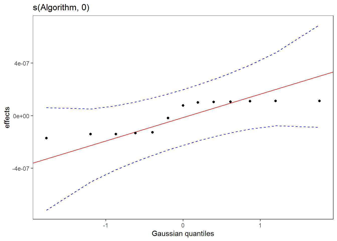

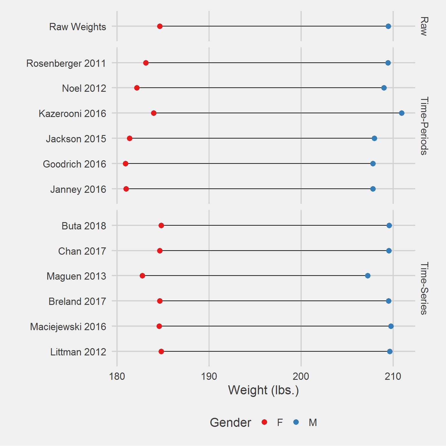
Distribution of weight measurements, by algorithm,

tmp <- DF %>%
  filter(!is.na(Weight)) %>%
  group_by(Type, Algorithm, Gender) %>%
  dplyr::summarise(
    weight_n = n(),
    mean     = mean(Weight),
    SD       = sd(Weight),
    median   = median(Weight),
    IQR      = IQR(Weight),
    min      = min(Weight),
    max      = max(Weight)
  )


tableStyle(tmp)

Type	Algorithm	Gender	weight_n	mean	SD	median	IQR	min	max
Raw	Raw Weights	F	78526	184.66	44.56	180.70	59.80	0.00	1479.90
Raw	Raw Weights	M	1097469	209.48	48.45	204.00	60.00	0.00	1486.20
Time-Periods	Janney 2016	F	12268	181.00	42.37	177.00	56.90	78.40	473.99
Time-Periods	Janney 2016	M	187562	207.80	45.17	202.55	56.20	80.00	546.00
Time-Periods	Goodrich 2016	F	12268	180.93	42.25	177.00	56.90	80.25	382.00
Time-Periods	Goodrich 2016	M	187518	207.78	45.13	202.50	56.20	80.00	500.00
Time-Periods	Jackson 2015	F	15479	181.36	42.24	177.00	57.63	75.63	375.00
Time-Periods	Jackson 2015	M	236022	207.94	45.24	202.70	56.19	78.00	553.00
Time-Periods	Kazerooni 2016	F	5094	183.98	43.26	180.20	59.00	75.62	467.38
Time-Periods	Kazerooni 2016	M	66867	210.90	47.76	205.70	59.80	0.00	1233.70
Time-Periods	Noel 2012	F	44332	182.17	42.61	178.00	57.71	72.90	467.38
Time-Periods	Noel 2012	M	638676	208.99	45.86	203.60	57.30	70.00	588.90
Time-Periods	Rosenberger 2011	F	14116	183.13	43.41	179.00	57.90	0.00	1144.00
Time-Periods	Rosenberger 2011	M	213099	209.44	45.95	204.00	57.00	0.00	1314.50
Time-Series	Littman 2012	F	77105	184.79	43.71	180.90	59.60	77.38	413.80
Time-Series	Littman 2012	M	1084556	209.62	48.02	204.00	59.73	75.20	546.00
Time-Series	Maciejewski 2016	F	77240	184.57	43.72	180.60	59.88	62.00	413.80
Time-Series	Maciejewski 2016	M	1067596	209.76	47.99	204.00	59.70	64.00	546.00
Time-Series	Breland 2017	F	78462	184.66	43.79	180.78	59.80	75.00	473.99
Time-Series	Breland 2017	M	1096715	209.51	48.12	204.00	59.90	75.20	694.46
Time-Series	Maguen 2013	F	69824	182.76	42.81	179.00	58.50	70.30	382.00
Time-Series	Maguen 2013	M	967469	207.23	46.18	202.00	57.90	74.00	541.10
Time-Series	Chan 2017	F	78150	184.66	43.82	180.80	59.80	59.20	725.32
Time-Series	Chan 2017	M	1091964	209.52	48.14	204.00	59.90	54.00	727.50
Time-Series	Buta 2018	F	76284	184.81	43.81	181.00	59.95	60.00	415.79
Time-Series	Buta 2018	M	1055712	209.58	48.17	204.00	60.00	66.50	540.00

tmp %>%
  ggplot(aes(mean, Algorithm)) %>%
  add(geom_line(aes(group = Algorithm))) %>%
  add(geom_point(aes(color = Gender), size = 3)) %>%
  add(facet_grid(rows = vars(Type), scales = "free", space = "free")) %>%
  add(theme_fivethirtyeight(16)) %>%
  add(theme(axis.title = element_text())) %>%
  add(scale_color_brewer(palette = "Set1")) %>%
  add(labs(
    x = "Weight (lbs.)",
    y = ""
  ))

Test/model if there is a difference by algorithm choice

test_mean <- mgcv::gam(
  mean ~ Gender + s(Algorithm, bs = 're'),
  data = tmp,
  family = gaussian,
  method = 'REML'
)

broom::tidy(test_mean)

# A tibble: 1 x 5
  term           edf ref.df statistic  p.value
  <chr>        <dbl>  <dbl>     <dbl>    <dbl>
1 s(Algorithm)  9.96     12      4.87 0.000569

This would suggest that there are some differences by Algorithm on the mean; mean weight is expected to differ by sex.

test_sd <- mgcv::gam(
  SD ~ Gender + s(Algorithm, bs = 're'),
  data = tmp,
  family = gaussian,
  method = 'REML'
)

broom::tidy(test_sd)

# A tibble: 1 x 5
  term           edf ref.df statistic   p.value
  <chr>        <dbl>  <dbl>     <dbl>     <dbl>
1 s(Algorithm)  10.5     12      7.03 0.0000380

And there certainly is some difference in standard deviation by algorithm

Number of Patients/Veterans Retained, by algorithm, by Sex,

tmp <- DF %>%
  filter(!is.na(Weight)) %>%
  group_by(Type, Algorithm, Gender) %>%
  distinct(PatientICN) %>%
  count()

tableStyle(tmp)

Type	Algorithm	Gender	n
Raw	Raw Weights	F	6200
Raw	Raw Weights	M	92758
Time-Periods	Janney 2016	F	5933
Time-Periods	Janney 2016	M	89809
Time-Periods	Goodrich 2016	F	5935
Time-Periods	Goodrich 2016	M	89811
Time-Periods	Jackson 2015	F	6007
Time-Periods	Jackson 2015	M	90552
Time-Periods	Kazerooni 2016	F	1698
Time-Periods	Kazerooni 2016	M	22289
Time-Periods	Noel 2012	F	6200
Time-Periods	Noel 2012	M	92758
Time-Periods	Rosenberger 2011	F	3929
Time-Periods	Rosenberger 2011	M	59476
Time-Series	Littman 2012	F	6026
Time-Series	Littman 2012	M	90104
Time-Series	Maciejewski 2016	F	6200
Time-Series	Maciejewski 2016	M	92758
Time-Series	Breland 2017	F	6200
Time-Series	Breland 2017	M	92758
Time-Series	Maguen 2013	F	6164
Time-Series	Maguen 2013	M	92188
Time-Series	Chan 2017	F	6027
Time-Series	Chan 2017	M	90105
Time-Series	Buta 2018	F	5749
Time-Series	Buta 2018	M	84410

tmp %>%
  ggplot(aes(x = Algorithm, y = n)) %>%
  add(geom_point(aes(fill = Gender), size = 4, pch = 21)) %>%
  add(facet_grid(
    cols = vars(Gender), 
    rows = vars(Type), 
    scales = "free",
    space = "free_y"
  )) %>%
  add(theme_fivethirtyeight(16)) %>%
  add(theme(axis.title = element_text())) %>%
  add(scale_fill_brewer(palette = "Set1")) %>%
  add(coord_flip()) %>%
  add(labs(
    x = "",
    y = "N Patients Retained"
  ))

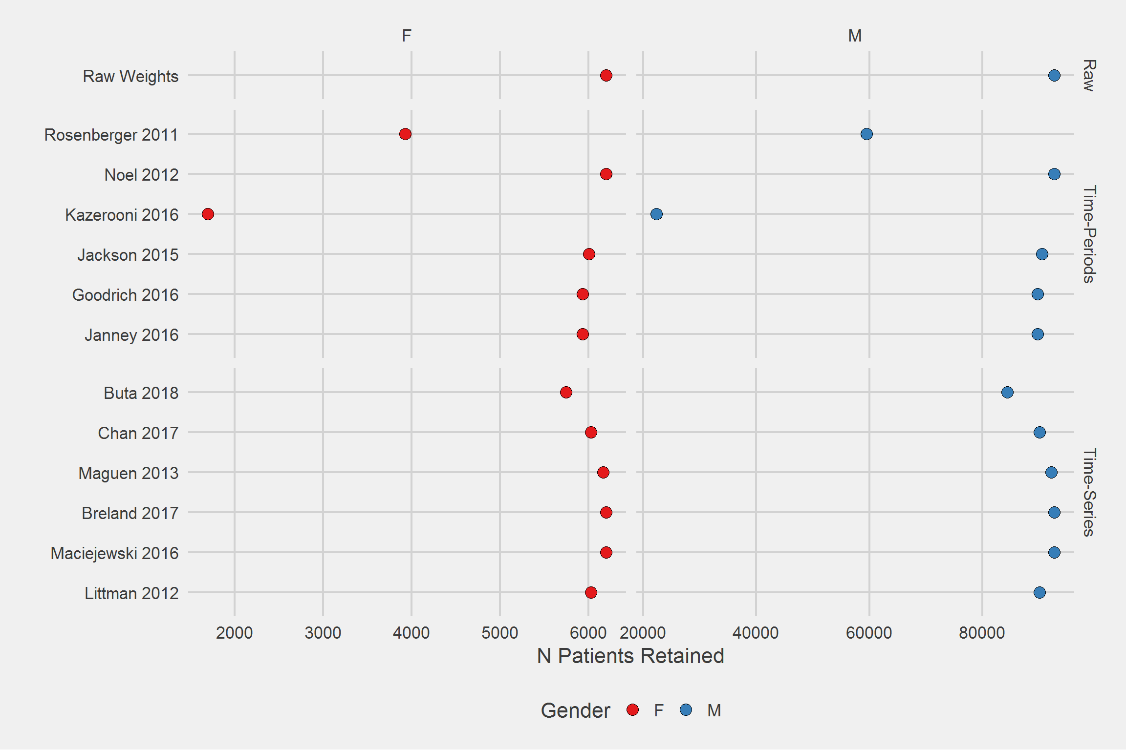
The relative differences in algorithmic effect between sexes are minute.

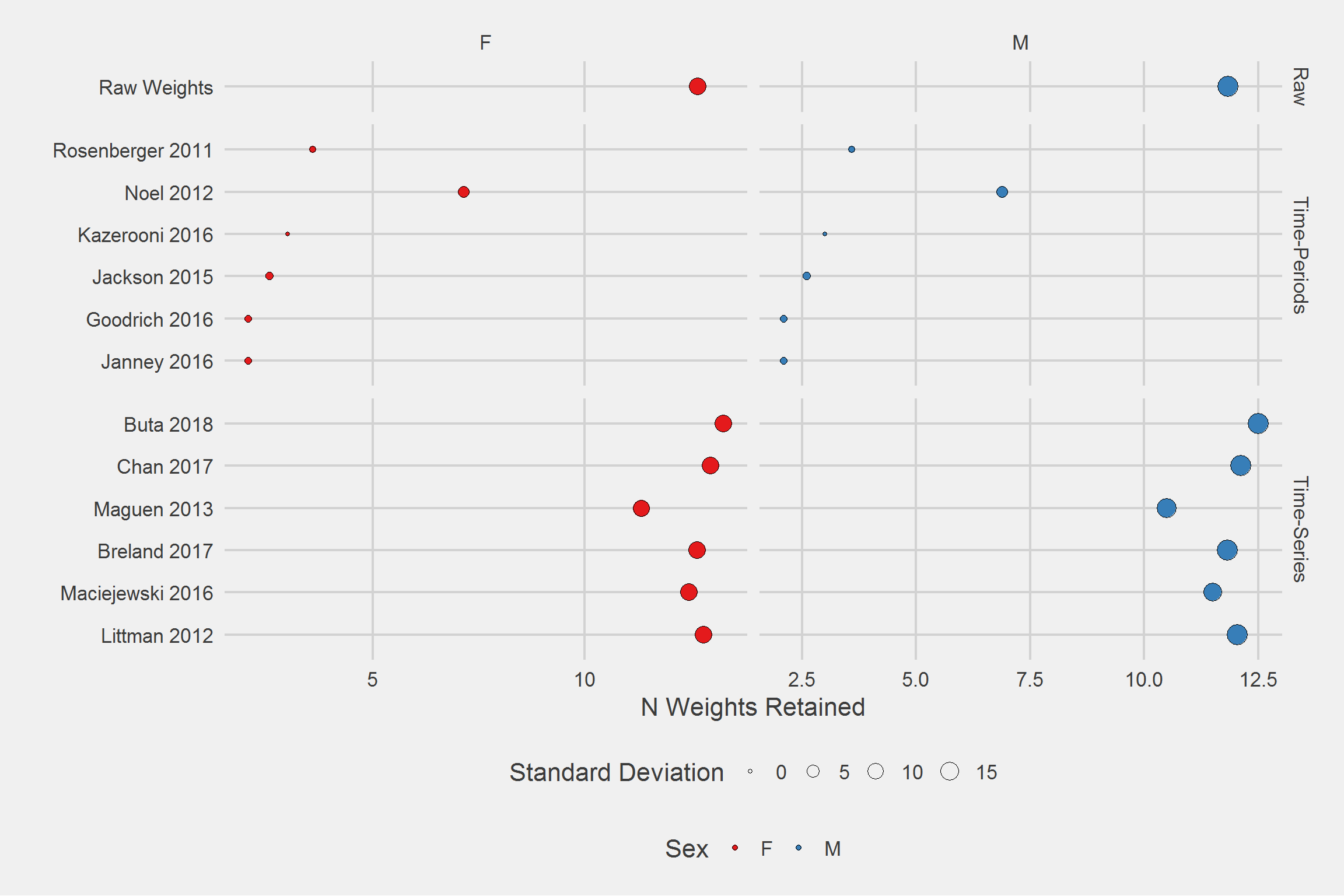
Number of weights retained, per person, by algorithm, by Sex,

tmp <- DF %>%
  filter(!is.na(Weight)) %>%
  group_by(Type, Algorithm, Gender, PatientICN) %>%
  count() %>%
  ungroup() %>%
  group_by(Type, Algorithm, Gender) %>%
  summarize(
    mean   = mean(n),
    SD     = sd(n),
    min    = min(n),
    Q1     = fivenum(n)[2],
    median = median(n),
    Q3     = fivenum(n)[4],
    max    = max(n)
  )

tableStyle(tmp)

Type	Algorithm	Gender	mean	SD	min	Q1	median	Q3	max
Raw	Raw Weights	F	12.67	12.61	1	5	9	16	277
Raw	Raw Weights	M	11.83	19.05	1	4	8	14	1525
Time-Periods	Janney 2016	F	2.07	0.78	1	1	2	3	3
Time-Periods	Janney 2016	M	2.09	0.76	1	2	2	3	3
Time-Periods	Goodrich 2016	F	2.07	0.78	1	1	2	3	3
Time-Periods	Goodrich 2016	M	2.09	0.76	1	2	2	3	3
Time-Periods	Jackson 2015	F	2.58	1.00	1	2	3	3	4
Time-Periods	Jackson 2015	M	2.61	0.98	1	2	3	3	4
Time-Periods	Kazerooni 2016	F	3.00	0.00	3	3	3	3	3
Time-Periods	Kazerooni 2016	M	3.00	0.00	3	3	3	3	3
Time-Periods	Noel 2012	F	7.15	3.75	1	4	7	10	17
Time-Periods	Noel 2012	M	6.89	3.72	1	4	6	9	17
Time-Periods	Rosenberger 2011	F	3.59	0.49	3	3	4	4	4
Time-Periods	Rosenberger 2011	M	3.58	0.49	3	3	4	4	4
Time-Series	Littman 2012	F	12.80	12.43	2	5	9	16	277
Time-Series	Littman 2012	M	12.04	19.11	2	5	8	14	1524
Time-Series	Maciejewski 2016	F	12.46	12.25	1	5	9	16	258
Time-Series	Maciejewski 2016	M	11.51	14.43	1	4	8	14	637
Time-Series	Breland 2017	F	12.66	12.61	1	5	9	16	277
Time-Series	Breland 2017	M	11.82	19.02	1	4	8	14	1524
Time-Series	Maguen 2013	F	11.33	10.89	1	5	8	14	192
Time-Series	Maguen 2013	M	10.49	16.91	1	4	7	13	1516
Time-Series	Chan 2017	F	12.97	12.56	2	5	9	16	269
Time-Series	Chan 2017	M	12.12	19.11	2	5	8	14	1517
Time-Series	Buta 2018	F	13.27	12.68	2	5	10	17	277
Time-Series	Buta 2018	M	12.51	19.73	2	5	8	15	1524

Testing/modeling

test_mean <- mgcv::gam(
  mean ~ Gender + Type + s(Algorithm, bs = 're'),
  data = tmp,
  family = gaussian,
  method = 'REML'
)

summary(test_mean)

Family: gaussian 
Link function: identity 

Formula:
mean ~ Gender + Type + s(Algorithm, bs = "re")

Parametric coefficients:
                 Estimate Std. Error t value Pr(>|t|)    
(Intercept)      12.48003    1.40738   8.868 1.13e-06 ***
GenderM          -0.46305    0.11716  -3.952  0.00185 ** 
TypeTime-Periods -8.85635    1.51882  -5.831 7.50e-05 ***
TypeTime-Series  -0.08501    1.51882  -0.056  0.95627    
---
Signif. codes:  0 '***' 0.001 '**' 0.01 '*' 0.05 '.' 0.1 ' ' 1

Approximate significance of smooth terms:
               edf Ref.df     F p-value    
s(Algorithm) 9.774     10 43.33  <2e-16 ***
---
Signif. codes:  0 '***' 0.001 '**' 0.01 '*' 0.05 '.' 0.1 ' ' 1

R-sq.(adj) =  0.996   Deviance explained = 99.8%
-REML = 27.358  Scale est. = 0.089217  n = 26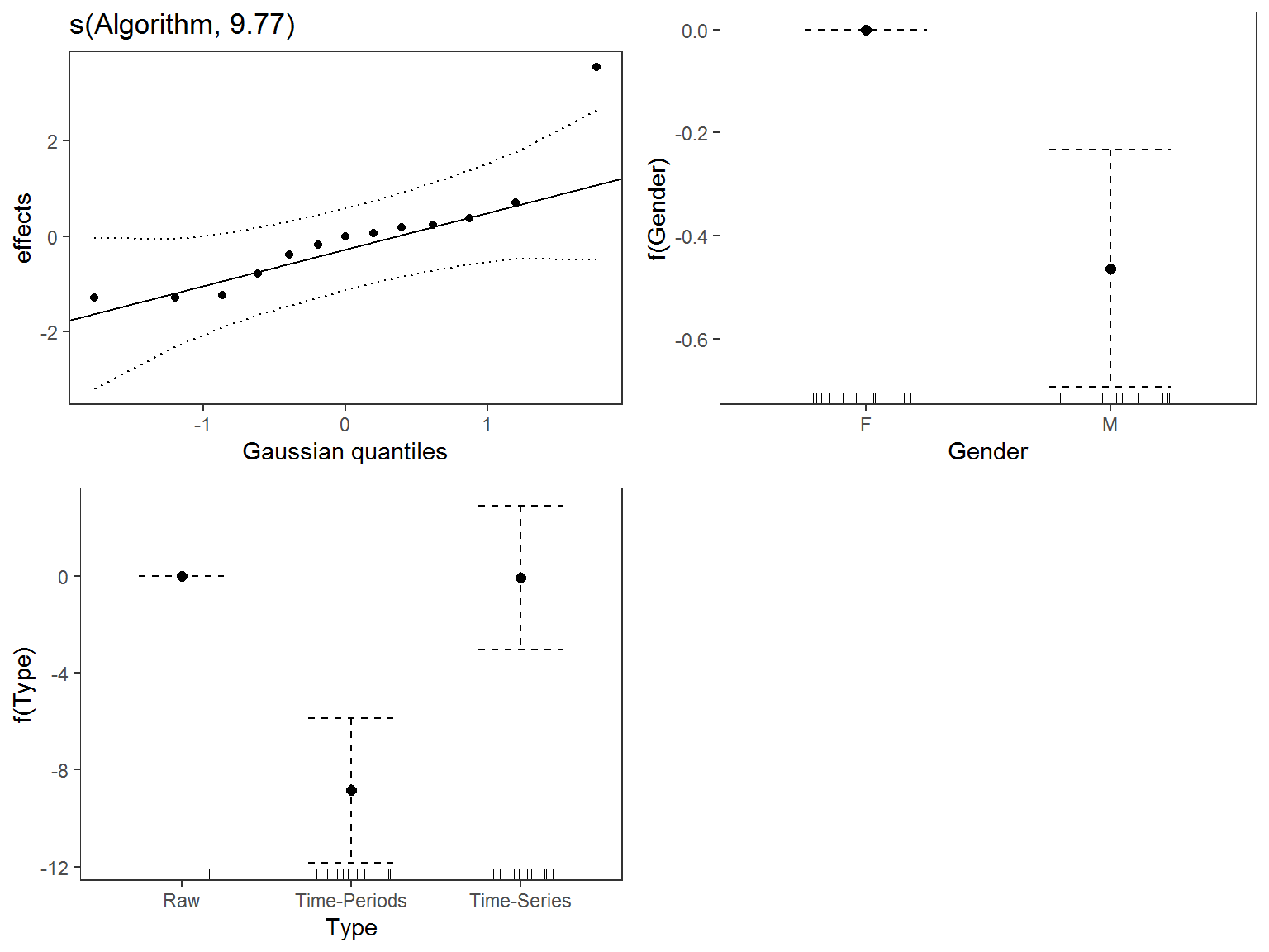

print(plot(getViz(test_mean), allTerms = TRUE), pages = 1)

These results suggest there are differences between algorithms and sex, though not for algorithms that use all data, at least when compared to the “raw” data.

tmp %>%
  ggplot(aes(x = Algorithm, y = mean)) %>%
  add(geom_point(aes(fill = Gender, size = SD), pch = 21)) %>%
  add(facet_grid(
    cols = vars(Gender), 
    rows = vars(Type), 
    scales = "free",
    space = "free_y"
  )) %>%
  add(theme_fivethirtyeight(16)) %>%
  add(theme(axis.title = element_text())) %>%
  add(scale_fill_brewer(palette = "Set1")) %>%
  add(coord_flip()) %>%
  add(labs(
    x = "",
    y = "N Weights Retained",
    size = "Standard Deviation",
    fill = "Sex"
  ))

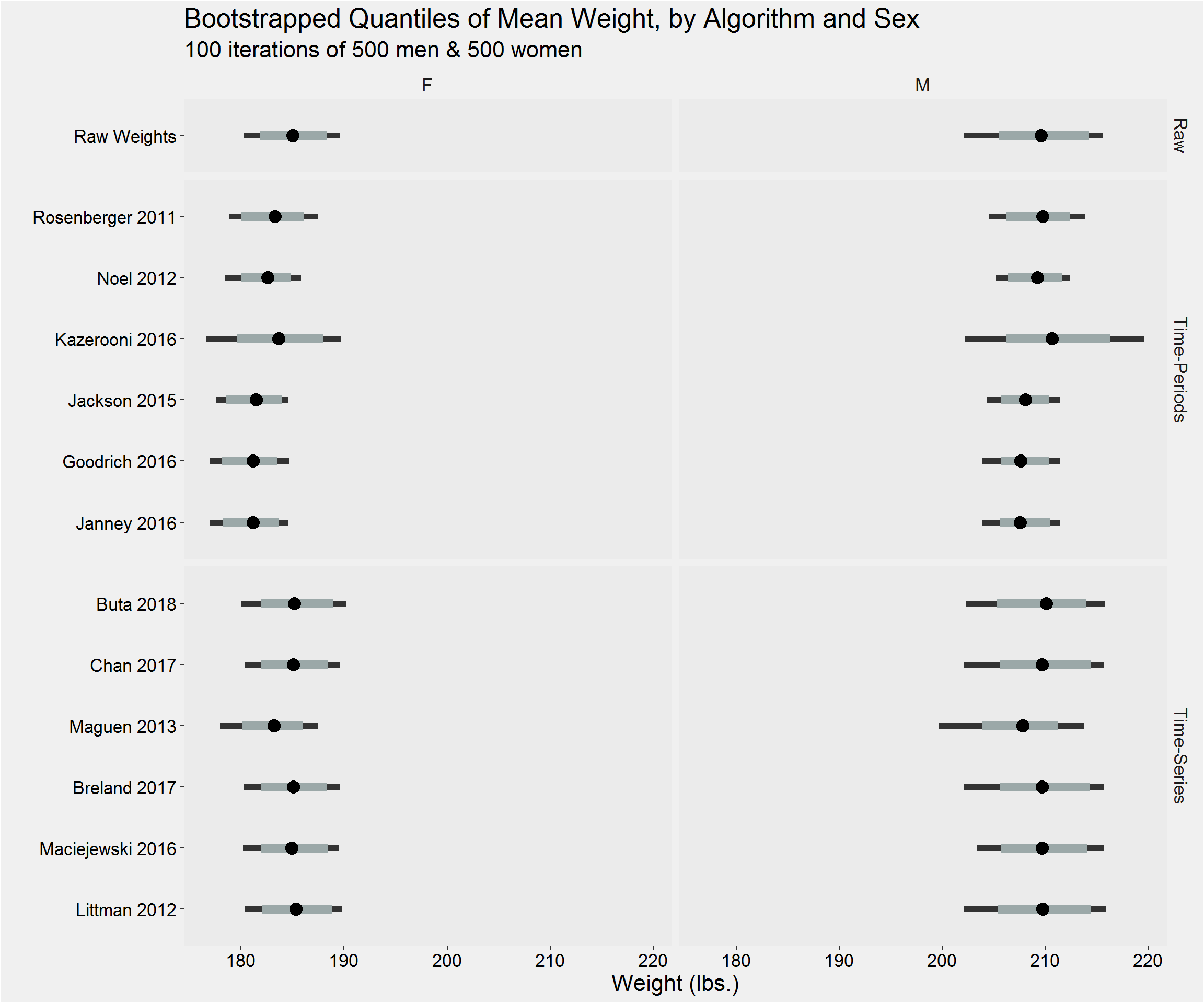
Bootstrapped Estimates

pts <- DF %>% distinct(PatientICN, Gender)

N <- 100
weight_samps <- vector("list", N)
key_cols <- c("Algorithm", "Gender")

pb <- txtProgressBar(min = 0, max = N, initial = 0, style = 3)

for (i in 1:N) {
  setTxtProgressBar(pb, i)
  sampM <- sample(
    pts %>% filter(Gender == "M") %>% pull(PatientICN),
    size = 500, 
    replace = TRUE
  )
  sampF <- sample(
    pts %>% filter(Gender == "F") %>% pull(PatientICN),
    size = 500,
    replace = TRUE
  )
  samp <- c(sampM, sampF)
  weight_samps[[i]] <- DF %>% filter(PatientICN %in% samp)
  setDT(weight_samps[[i]])
  setkeyv(weight_samps[[i]], key_cols)
  weight_samps[[i]] <- 
    weight_samps[[i]][, 
                      list(mean = mean(Weight), SD = sd(Weight)), 
                      by = key_cols
                      ]
}

Visualization

Distribution of the mean

Distribution of the sample standard deviation

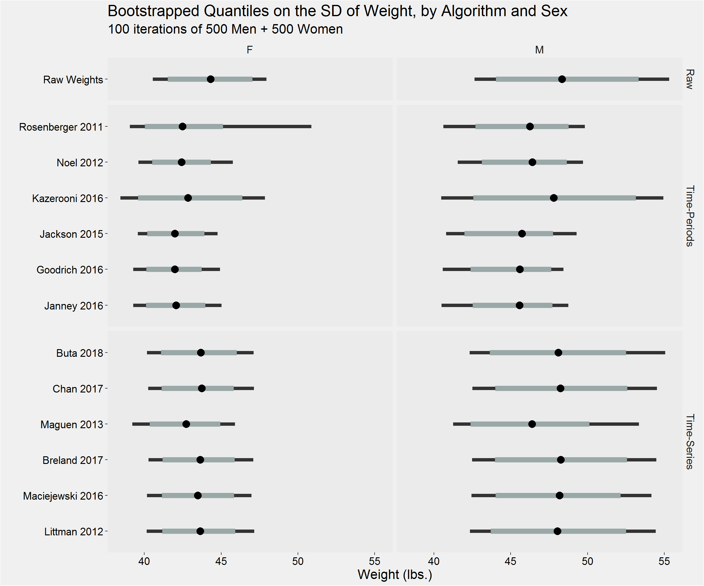
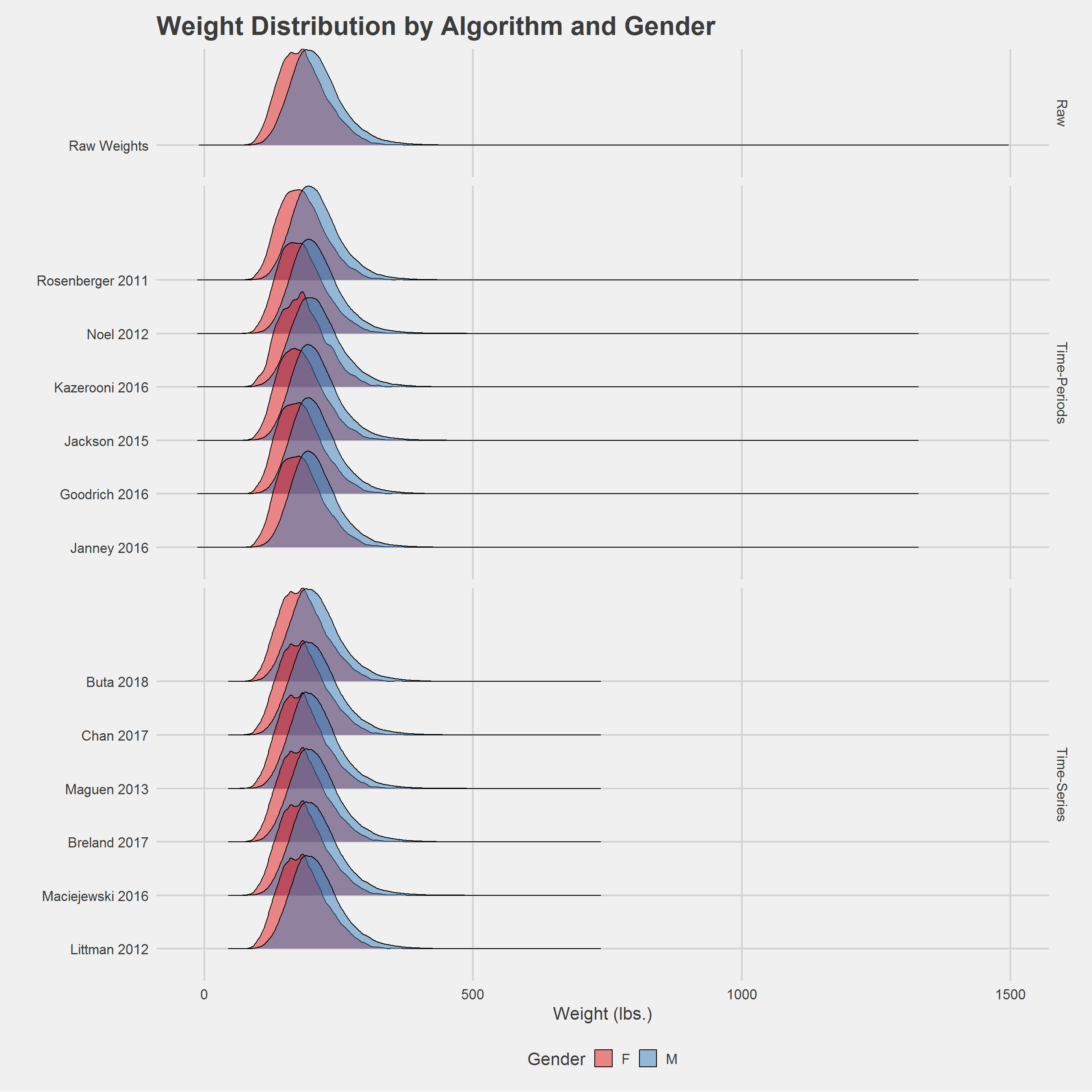
Alternative, ridgeline plot

Latent Trajectories

Sampling 500 men & 500 women from the PCP 2016 Cohort

library(lcmm)

# variable 'subject' must be numeric
for (i in 1:length(me)) {
  if (class(me[[i]]$PatientICN) == "factor") {
    me[[i]]$PatientICN <- as.integer(as.character(me[[i]]$PatientICN))
  }
}

# initial values/model
B_M <- lcmm(
  Weight ~ time,
  random = ~time,
  subject = "PatientICN",
  ng = 1,
  idiag = TRUE,
  data = me[[1]] %>% filter(Gender == "M"),
  verbose = TRUE
)

B_F <- lcmm(
  Weight ~ time,
  random = ~time,
  subject = "PatientICN",
  ng = 1,
  idiag = TRUE,
  data = me[[1]] %>% filter(Gender == "F"),
  verbose = TRUE
)

lca.mods.M <- lapply(
  me,
  FUN = function(x) {
    lcmm(
      Weight ~ time,
      random = ~time,
      subject = "PatientICN",
      mixture = ~time,
      ng = 3,
      idiag = TRUE,
      data = x %>% filter(Gender == "M"),
      B = B_M
    )
  }
)

lca.mods.F <- lapply(
  me,
  FUN = function(x) {
    lcmm(
      Weight ~ time,
      random = ~time,
      subject = "PatientICN",
      mixture = ~time,
      ng = 3,
      idiag = TRUE,
      data = x %>% filter(Gender == "F"),
      B = B_F
    )
  }
)

names(lca.mods.M) <- names(me)
for (i in 1:length(lca.mods.M)) {
  lca.mods.M[[i]]$data <- me[[i]] %>% filter(Gender == "M")
}

names(lca.mods.F) <- names(me)
for (i in 1:length(lca.mods.F)) {
  lca.mods.F[[i]]$data <- me[[i]] %>% filter(Gender == "F")
}

Predicted classes

So, there is no guarantee that each class within an algorithms LCMM, will be the same class across algorithms. We can get this information from the signs of the coefficients on “time” in each model.

concept_classes <- c("Loss", "Maintain", "Gain")

traj_edies_M <- sapply(
  lca.mods.M,
  function(x) {
    time_coefs <- coef(x)
    which_coef <- grepl("time", names(time_coefs))
    time_coefs <- time_coefs[which_coef]
    traj_class <- sign(round(time_coefs, 3))
    traj_class
  }
) %>%
  as.data.frame() %>% 
  rownames_to_column("orig_class") %>% 
  pivot_longer(
    !orig_class, 
    names_to = "Algorithm", 
    values_to = "value"
  ) %>%
  mutate(
    Algorithm = factor(Algorithm,
                       levels = names(me),
                       labels = names(me)),
    concept_class = case_when(
      value == -1 ~ concept_classes[1],
      value == 0  ~ concept_classes[2],
      value == 1  ~ concept_classes[3]
    ),
    concept_class = factor(
      concept_class,
      levels = concept_classes,
      labels = concept_classes
    ),
    orig_class = case_when(
      orig_class == "time class1" ~ "Class 1",
      orig_class == "time class2" ~ "Class 2",
      orig_class == "time class3" ~ "Class 3"
    ),
    orig_class = factor(orig_class)
  ) %>%
  select(-value) %>%
  distinct(Algorithm, concept_class, .keep_all = TRUE)

traj_edies_F <- sapply(
  lca.mods.F,
  function(x) {
    time_coefs <- coef(x)
    which_coef <- grepl("time", names(time_coefs))
    time_coefs <- time_coefs[which_coef]
    traj_class <- sign(round(time_coefs, 3))
    traj_class
  }
) %>%
  as.data.frame() %>% 
  rownames_to_column("orig_class") %>% 
  pivot_longer(
    !orig_class, 
    names_to = "Algorithm", 
    values_to = "value"
  ) %>%
  mutate(
    Algorithm = factor(Algorithm,
                       levels = names(me),
                       labels = names(me)),
    concept_class = case_when(
      value == -1 ~ concept_classes[1],
      value == 0  ~ concept_classes[2],
      value == 1  ~ concept_classes[3]
    ),
    concept_class = factor(
      concept_class,
      levels = concept_classes,
      labels = concept_classes
    ),
    orig_class = case_when(
      orig_class == "time class1" ~ "Class 1",
      orig_class == "time class2" ~ "Class 2",
      orig_class == "time class3" ~ "Class 3"
    ),
    orig_class = factor(orig_class)
  ) %>%
  select(-value) %>%
  distinct(Algorithm, concept_class, .keep_all = TRUE)

newdata <- data.frame(time = seq(0, 365, 5))

Ypred_lcmm.M <- lapply(
  lca.mods.M,
  function(x) {
    y <- predictY(x, newdata, var.time = "time")
    cbind(y$pred, y$time)
   }
) %>%
  dplyr::bind_rows(.id = "Algorithm") %>%
  pivot_longer(
    !c(Algorithm, time), 
    names_to = "orig_class", 
    values_to = "Ypred"
  ) %>%
  mutate(
    Algorithm = factor(Algorithm,
                       levels = names(me),
                       labels = names(me)),
    orig_class = factor(orig_class,
                        levels = c("Ypred_class1", "Ypred_class2", "Ypred_class3"),
                        labels = c("Class 1", "Class 2", "Class 3"))
  ) %>%
  left_join(
    traj_edies_M,
    by = c("Algorithm", "orig_class")
  ) %>%
  na.omit()

Ypred_lcmm.F <- lapply(
  lca.mods.F,
  function(x) {
    y <- predictY(x, newdata, var.time = "time")
    cbind(y$pred, y$time)
   }
) %>%
  dplyr::bind_rows(.id = "Algorithm") %>%
  pivot_longer(
    !c(Algorithm, time), 
    names_to = "orig_class", 
    values_to = "Ypred"
  ) %>%
  mutate(
    Algorithm = factor(Algorithm,
                       levels = names(me),
                       labels = names(me)),
    orig_class = factor(orig_class,
                        levels = c("Ypred_class1", "Ypred_class2", "Ypred_class3"),
                        labels = c("Class 1", "Class 2", "Class 3"))
  ) %>%
  left_join(
    traj_edies_F,
    by = c("Algorithm", "orig_class")
  ) %>%
  na.omit()

Ypred_lcmm <- bind_rows(
  `Males`   = Ypred_lcmm.M,
  `Females` = Ypred_lcmm.F,
  .id = "Sex"
)

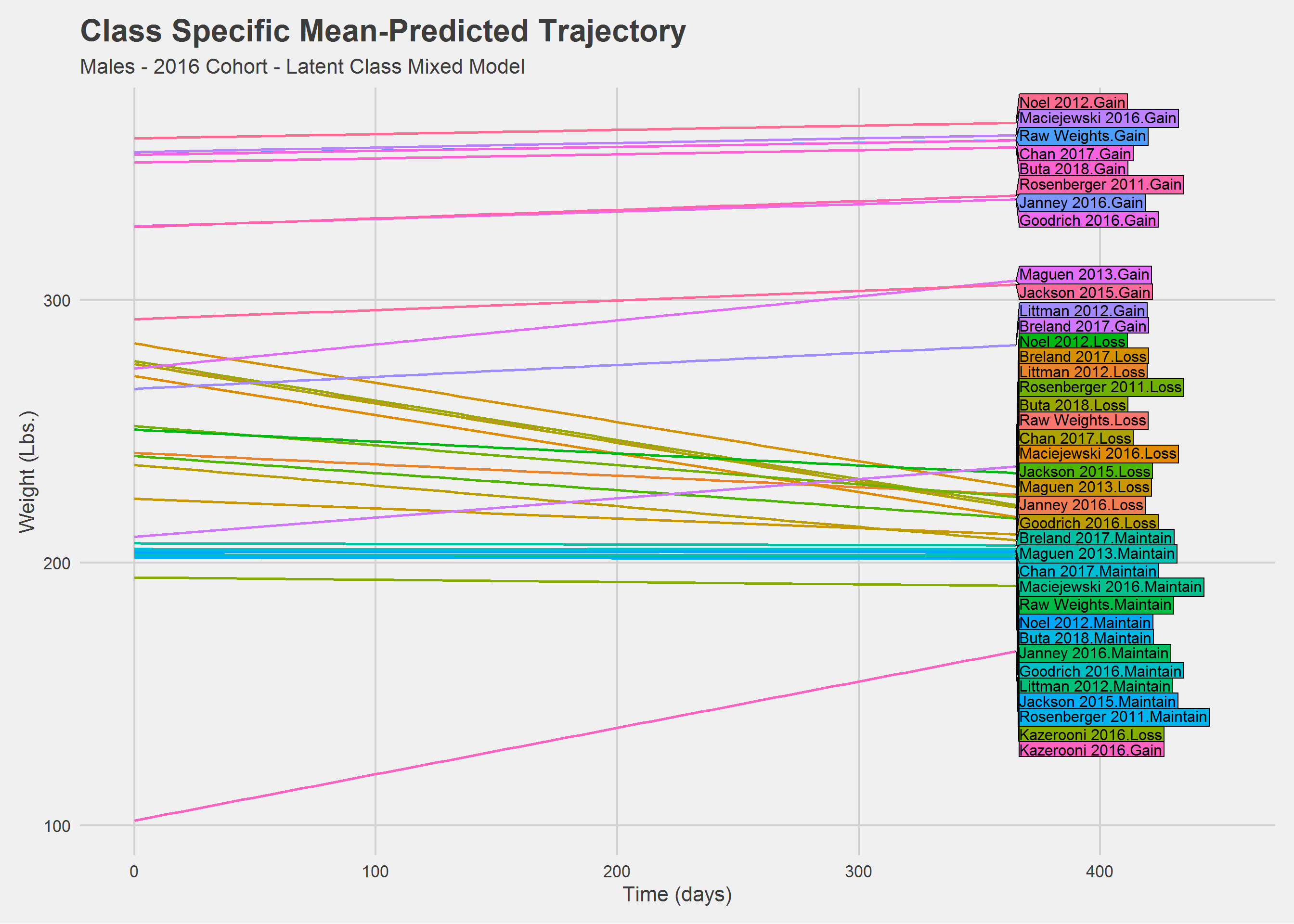
rm(Ypred_lcmm.M, Ypred_lcmm.F)

Men

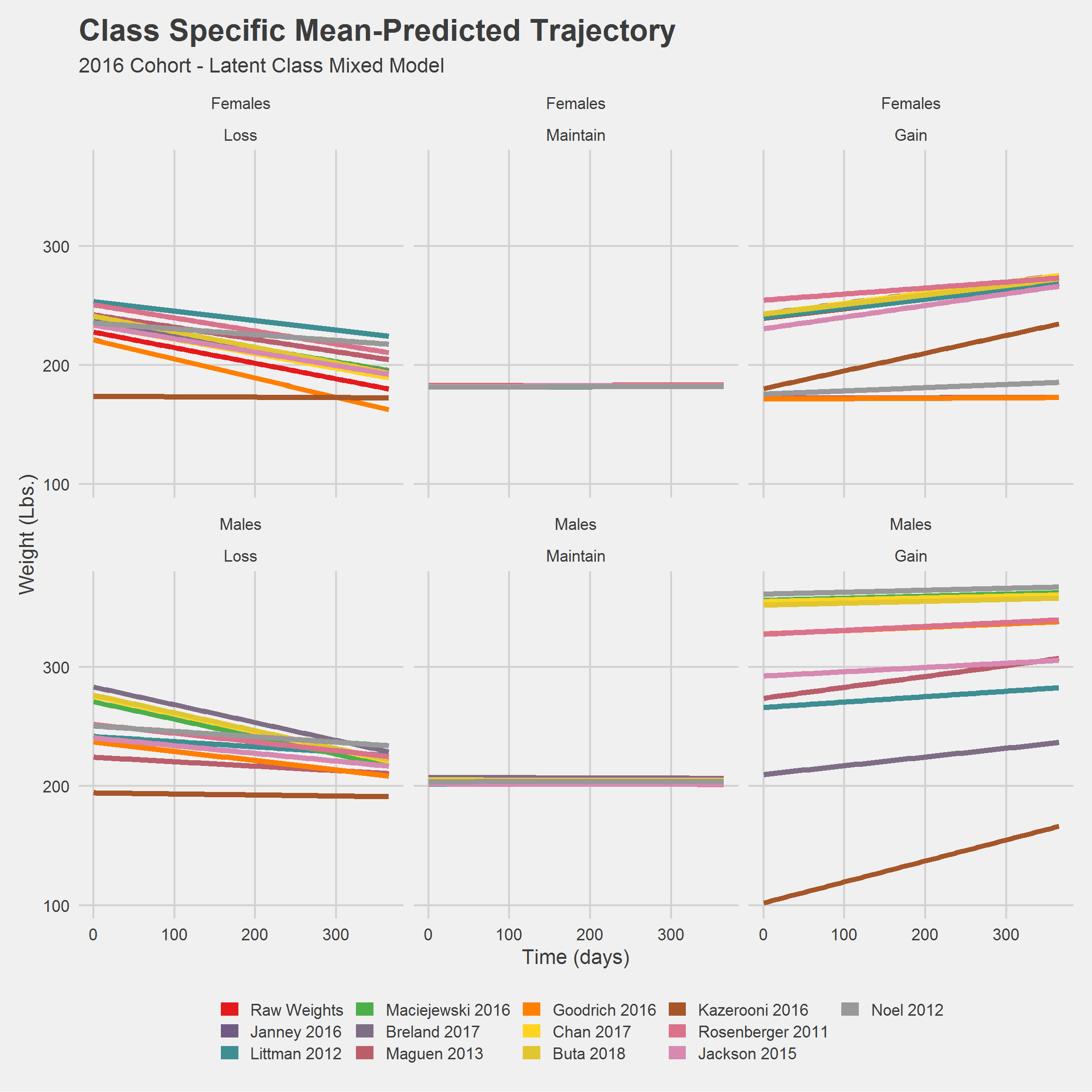
Ypred_lcmm %>%
  filter(Sex == "Males") %>%
  ggplot(
    aes(
      x = time, y = Ypred,
      group = interaction(Algorithm, concept_class),
      color = interaction(Algorithm, concept_class)
    )
  ) %>%
  add(geom_line(size = 1)) %>%
  add(theme_fivethirtyeight(16)) %>%
  add(theme(axis.title = element_text(), legend.position = "none")) %>%
  add(xlim(0, 450)) %>% 
  add(directlabels::geom_dl(aes(label = interaction(Algorithm, concept_class)),
                            method = "last.polygons")) %>%
  add(labs(
    x = "Time (days)",
    y = "Weight (Lbs.)",
    title = "Class Specific Mean-Predicted Trajectory",
    subtitle = "Males - 2016 Cohort - Latent Class Mixed Model",
    color = ""
  ))

Women

Ypred_lcmm %>%
  filter(Sex == "Females") %>%
  ggplot(
    aes(
      x = time, y = Ypred,
      group = interaction(Algorithm, concept_class),
      color = interaction(Algorithm, concept_class)
    )
  ) %>%
  add(geom_line(size = 1)) %>%
  add(theme_fivethirtyeight(16)) %>%
  add(theme(axis.title = element_text(), legend.position = "none")) %>%
  add(xlim(0, 450)) %>% 
  add(directlabels::geom_dl(aes(label = interaction(Algorithm, concept_class)),
                            method = "last.polygons")) %>%
  add(labs(
    x = "Time (days)",
    y = "Weight (Lbs.)",
    title = "Class Specific Mean-Predicted Trajectory",
    subtitle = "Females - 2016 Cohort - Latent Class Mixed Model",
    color = ""
  ))

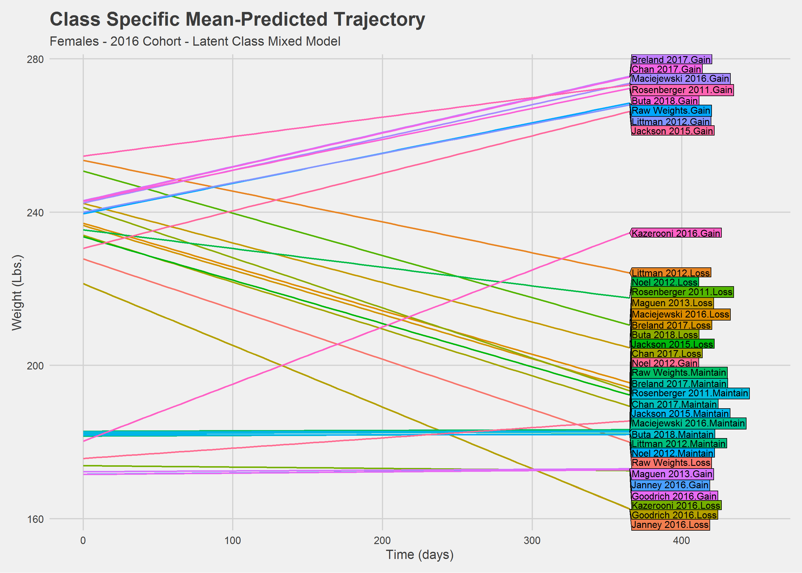
Still a mess. Let’s look at things a little differently.

An Illustration:

library(gganimate)

Ypred_lcmm %>%
  ggplot(
    aes(
      x = time,
      y = Ypred,
      color = Algorithm,
      group = interaction(Algorithm, concept_class)
    )
  ) %>%
  add(geom_line(size = 1)) %>%
  add(facet_wrap(vars(Sex))) %>%
  add(theme_minimal(20)) %>%
  add(theme(legend.position = "none")) %>%
  add(labs(
    title = 'Algorithm: {closest_state}',
    x = "Time (days)",
    y = "Weight (lbs.)"
  )) %>%
  add(transition_states(
    states = Algorithm,
    transition_length = 1,
    state_length = 2
  ))

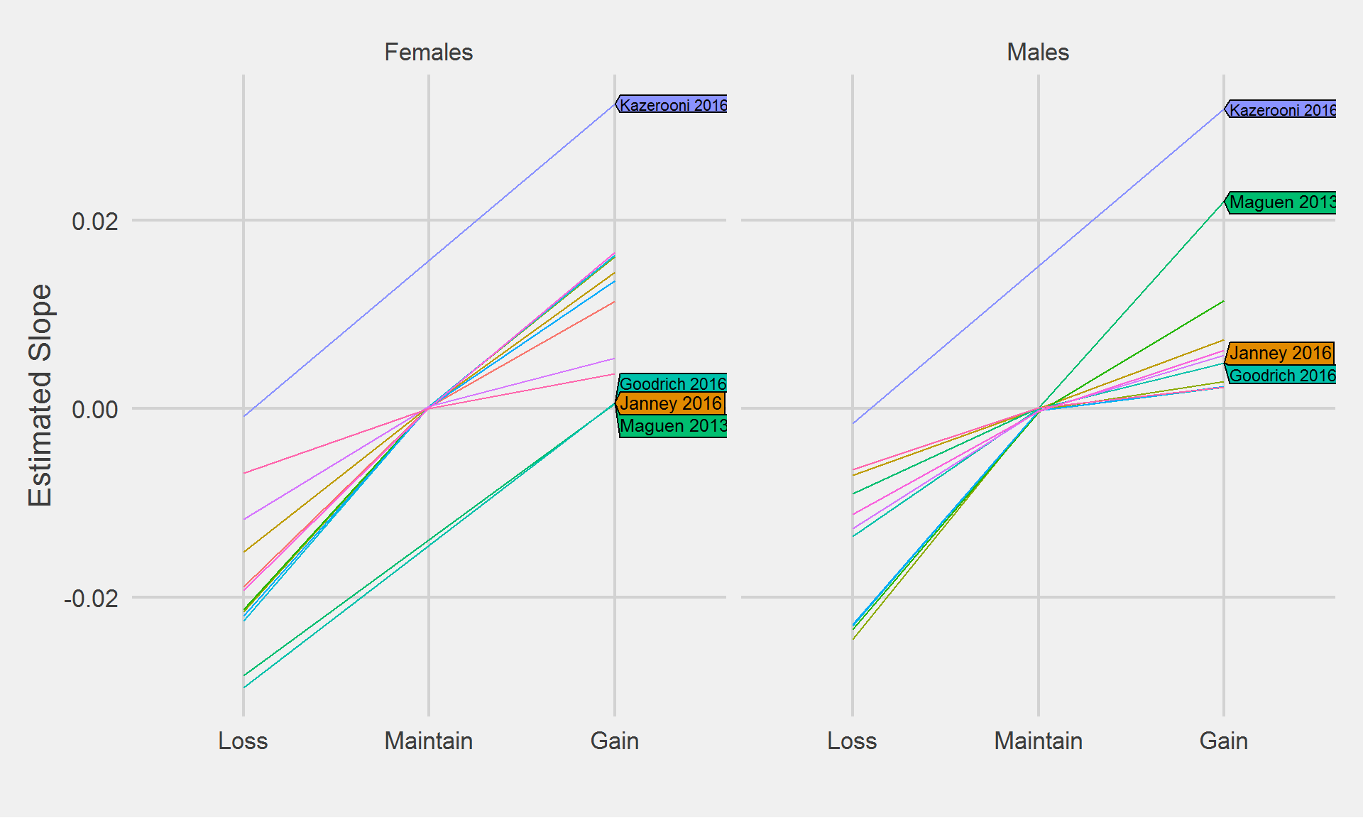
Comparing slopes, numerically

slopes.M <- sapply(
  lca.mods.M,
  function(x) {
    time_coefs <- coef(x)
    which_coef <- grepl("time", names(time_coefs))
    time_coefs <- time_coefs[which_coef]
    time_coefs <- round(time_coefs, 5)
    time_coefs
  }
) %>%
  reshape2::melt() %>%
  mutate(
    orig_class = case_when(
      Var1 == "time class1" ~ "Class 1",
      Var1 == "time class2" ~ "Class 2",
      Var1 == "time class3" ~ "Class 3"
    ),
    orig_class = factor(orig_class)
  ) %>%
  select(-Var1) %>%
  rename(Algorithm  = Var2, Slope = value) %>% 
  full_join(traj_edies_M, by = c("Algorithm", "orig_class"))

slopes.F <- sapply(
  lca.mods.F,
  function(x) {
    time_coefs <- coef(x)
    which_coef <- grepl("time", names(time_coefs))
    time_coefs <- time_coefs[which_coef]
    time_coefs <- round(time_coefs, 5)
    time_coefs
  }
) %>%
  reshape2::melt() %>%
  mutate(
    orig_class = case_when(
      Var1 == "time class1" ~ "Class 1",
      Var1 == "time class2" ~ "Class 2",
      Var1 == "time class3" ~ "Class 3"
    ),
    orig_class = factor(orig_class)
  ) %>%
  select(-Var1) %>%
  rename(Algorithm  = Var2, Slope = value) %>% 
  full_join(traj_edies_F, by = c("Algorithm", "orig_class"))

slopes <- bind_rows(
  `Males` = slopes.M,
  `Females` = slopes.F,
  .id = "Sex"
) %>% 
  na.omit()

rm(slopes.M, slopes.F)

algos <- c("Janney 2016", "Goodrich 2016", "Maguen 2013", "Kazerooni 2016")

slopes %>%
  ggplot(aes(
    x = concept_class,
    y = Slope,
    group = Algorithm,
    color = Algorithm
  )) %>%
  add(geom_line()) %>%
  add(facet_wrap(vars(Sex))) %>%
  add(directlabels::geom_dl(
    data = slopes %>%
      filter(Algorithm %in% algos),
    aes(label = Algorithm),
    method = list("last.polygons")
  )) %>%
  add(theme_fivethirtyeight(16)) %>%
  add(theme(legend.position = "none", axis.title = element_text())) %>%
  add(labs(
    x = "",
    y = "Estimated Slope"
  ))

Weight Change Comparison

Add Gender/Sex

DF <- DF %>%
  filter(Cohort == "PCP 2016") %>%
  left_join(
    weight.ls[["PCP2016"]] %>%
      distinct(PatientICN, Gender),
    by = "PatientICN"
  )

Individual Level

Let’s look at the proportions of weight loss \(\geq5\)% from baseline, by algorithm:

tmp <- DF %>%
  count(Algorithm, Gender, gt5perc_weightloss) %>%
  group_by(Algorithm, Gender) %>%
  mutate(prop = prop.table(n)) %>%
  filter(gt5perc_weightloss == 1) %>%
  select(-gt5perc_weightloss) 

tableStyle(tmp)

Algorithm	Gender	n	prop
Raw Weights	F	535	0.15
Raw Weights	M	7627	0.13
Janney 2016	F	509	0.15
Janney 2016	M	7333	0.13
Littman 2012	F	502	0.15
Littman 2012	M	7349	0.13
Maciejewski 2016	F	514	0.15
Maciejewski 2016	M	7471	0.14
Breland 2017	F	529	0.15
Breland 2017	M	7595	0.13
Maguen 2013	F	355	0.12
Maguen 2013	M	4578	0.09
Goodrich 2016	F	508	0.15
Goodrich 2016	M	7320	0.13
Chan 2017	F	523	0.15
Chan 2017	M	7546	0.13
Jackson 2015	F	503	0.15
Jackson 2015	M	7470	0.13
Buta 2018	F	515	0.15
Buta 2018	M	7247	0.14
Kazerooni 2016	F	228	0.13
Kazerooni 2016	M	3127	0.14
Noel 2012	F	515	0.15
Noel 2012	M	7271	0.13
Rosenberger 2011	F	356	0.16
Rosenberger 2011	M	5069	0.14

Testing/modeling

test_prop <- mgcv::gam(
  prop ~ Gender + s(Algorithm, bs = 're'),
  data = tmp,
  family = binomial,
  method = 'REML'
)

summary(test_prop)

Family: binomial 
Link function: logit 

Formula:
prop ~ Gender + s(Algorithm, bs = "re")

Parametric coefficients:
            Estimate Std. Error z value Pr(>|z|)  
(Intercept)  -1.7528     0.7817  -2.242   0.0249 *
GenderM      -0.1380     1.1340  -0.122   0.9032  
---
Signif. codes:  0 '***' 0.001 '**' 0.01 '*' 0.05 '.' 0.1 ' ' 1

Approximate significance of smooth terms:
                   edf Ref.df Chi.sq p-value
s(Algorithm) 7.222e-06     12      0       1

R-sq.(adj) =  0.333   Deviance explained = 34.3%
-REML = 2.5266  Scale est. = 1         n = 26

When factoring in Algorithm, the differences in weight loss proportion between sexes is insignificant

plot(sm(getViz(test_prop), 1)) %>%
  add(l_fitLine(color = "red")) %>%
  add(l_ciLine(mul = 5, color = "blue", linetype = 2)) %>% 
  add(l_points())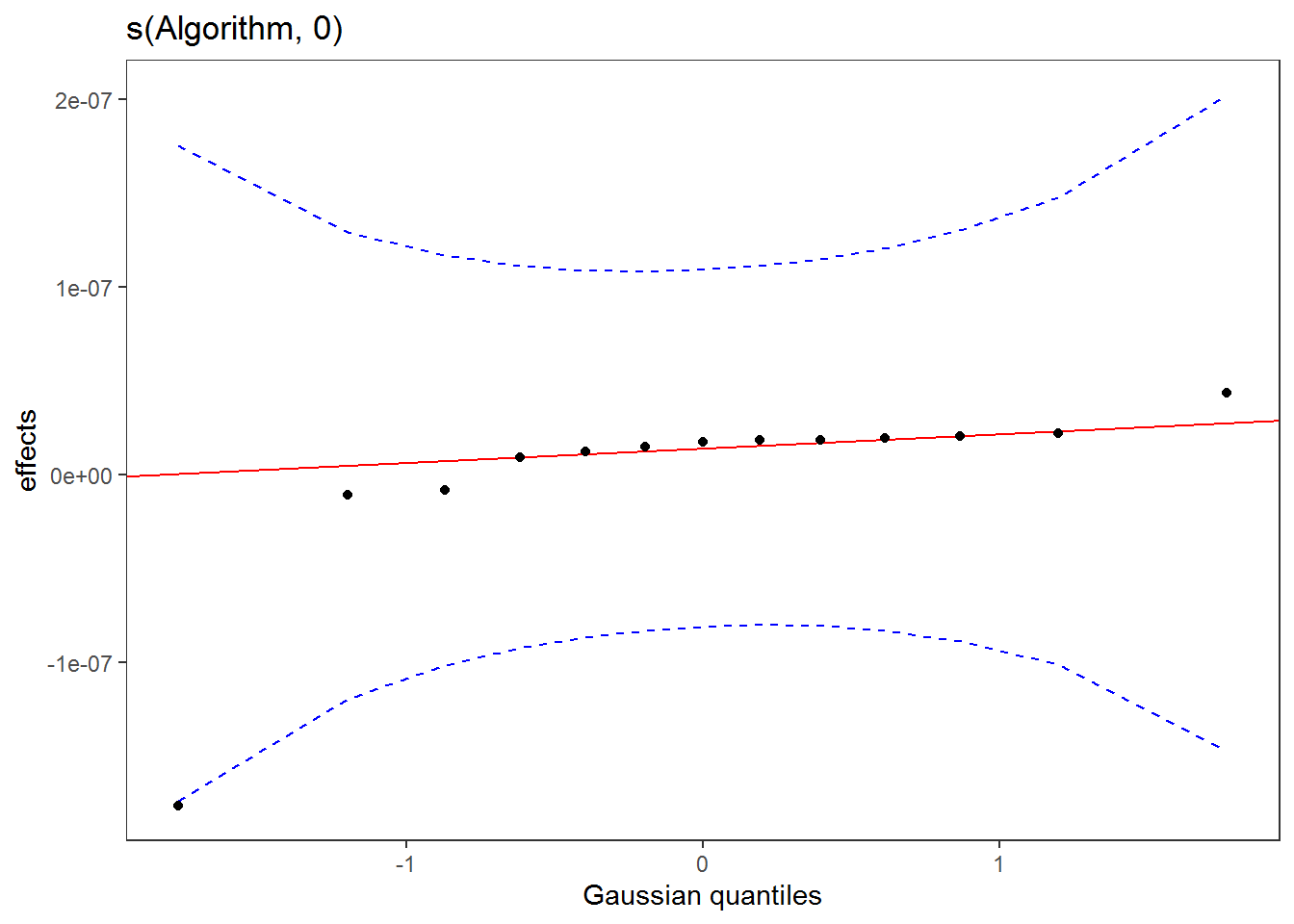

Let’s look at the proportions of weight gain \(\geq5\)% from baseline, by algorithm:

tmp <- DF %>%
  count(Algorithm, Gender, gt5perc_weightgain) %>%
  group_by(Algorithm, Gender) %>%
  mutate(prop = prop.table(n)) %>%
  filter(gt5perc_weightgain == 1) %>%
  select(-gt5perc_weightgain)

tableStyle(tmp)

Algorithm	Gender	n	prop
Raw Weights	F	626	0.18
Raw Weights	M	6351	0.11
Janney 2016	F	590	0.18
Janney 2016	M	6089	0.11
Littman 2012	F	603	0.17
Littman 2012	M	6184	0.11
Maciejewski 2016	F	620	0.18
Maciejewski 2016	M	6190	0.11
Breland 2017	F	624	0.18
Breland 2017	M	6312	0.11
Maguen 2013	F	425	0.14
Maguen 2013	M	3663	0.07
Goodrich 2016	F	590	0.18
Goodrich 2016	M	6078	0.11
Chan 2017	F	624	0.18
Chan 2017	M	6278	0.11
Jackson 2015	F	574	0.18
Jackson 2015	M	5920	0.10
Buta 2018	F	606	0.18
Buta 2018	M	6036	0.11
Kazerooni 2016	F	247	0.15
Kazerooni 2016	M	2256	0.10
Noel 2012	F	615	0.18
Noel 2012	M	6009	0.11
Rosenberger 2011	F	426	0.19
Rosenberger 2011	M	4299	0.12

Average weight change:

tmp <- DF %>%
  filter(!is.na(diff)) %>%
  select(Algorithm, Gender, diff) %>%
  group_by(Algorithm, Gender) %>%
  summarize(
    mean   = mean(diff),
    SD     = sd(diff),
    min    = min(diff),
    Q1     = fivenum(diff)[2],
    median = median(diff),
    Q3     = fivenum(diff)[4],
    max    = max(diff)
  )

tableStyle(tmp)

Algorithm	Gender	mean	SD	min	Q1	median	Q3	max
Raw Weights	F	-0.21	22.35	-1000.00	-5.20	0.56	6.40	185.00
Raw Weights	M	-0.65	13.27	-536.00	-5.70	-0.20	5.00	296.10
Janney 2016	F	0.07	13.84	-258.99	-5.25	0.59	6.30	98.40
Janney 2016	M	-0.65	11.91	-291.40	-5.70	-0.20	5.00	281.97
Littman 2012	F	0.45	11.36	-65.70	-5.00	0.60	6.30	88.90
Littman 2012	M	-0.55	10.72	-118.60	-5.60	-0.20	5.00	108.00
Maciejewski 2016	F	0.37	12.03	-95.30	-5.40	0.70	6.70	66.40
Maciejewski 2016	M	-0.67	11.21	-117.20	-5.90	-0.20	5.00	195.80
Breland 2017	F	0.20	13.07	-258.99	-5.20	0.60	6.40	88.90
Breland 2017	M	-0.65	11.44	-117.20	-5.70	-0.20	5.00	207.20
Maguen 2013	F	0.45	8.38	-42.00	-4.30	0.51	5.40	41.20
Maguen 2013	M	-0.42	7.74	-73.20	-4.90	-0.20	4.00	98.40
Goodrich 2016	F	0.21	12.57	-95.30	-5.20	0.59	6.30	98.40
Goodrich 2016	M	-0.65	11.44	-117.20	-5.70	-0.20	5.00	205.20
Chan 2017	F	0.27	12.85	-258.99	-5.10	0.60	6.40	98.40
Chan 2017	M	-0.63	11.89	-509.50	-5.70	-0.20	5.00	278.27
Jackson 2015	F	0.21	12.26	-133.50	-5.30	0.78	6.30	98.40
Jackson 2015	M	-0.76	11.25	-245.59	-5.80	-0.40	4.70	230.39
Buta 2018	F	0.16	13.32	-211.59	-5.20	0.60	6.40	98.40
Buta 2018	M	-0.64	11.92	-245.37	-5.80	-0.20	5.00	278.27
Kazerooni 2016	F	0.48	10.63	-84.00	-4.30	0.80	6.00	92.90
Kazerooni 2016	M	-1.06	12.56	-534.00	-6.20	-0.70	4.60	299.30
Noel 2012	F	0.25	12.87	-211.79	-5.25	0.65	6.53	98.40
Noel 2012	M	-0.63	11.39	-245.59	-5.70	-0.20	5.00	195.80
Rosenberger 2011	F	0.03	25.07	-1002.40	-5.55	0.80	7.00	185.00
Rosenberger 2011	M	-0.72	13.17	-538.00	-6.00	-0.30	5.00	298.70

Testing/modeling

test_mean <- mgcv::gam(
  mean ~ Gender + s(Algorithm, bs = 're'),
  data = tmp,
  family = gaussian,
  method = 'REML'
)

summary(test_mean)

Family: gaussian 
Link function: identity 

Formula:
mean ~ Gender + s(Algorithm, bs = "re")

Parametric coefficients:
            Estimate Std. Error t value Pr(>|t|)    
(Intercept)  0.22586    0.04709   4.796 6.98e-05 ***
GenderM     -0.89325    0.06660 -13.412 1.21e-12 ***
---
Signif. codes:  0 '***' 0.001 '**' 0.01 '*' 0.05 '.' 0.1 ' ' 1

Approximate significance of smooth terms:
                   edf Ref.df F p-value
s(Algorithm) 4.182e-05     12 0   0.527

R-sq.(adj) =  0.877   Deviance explained = 88.2%
-REML = -5.9358  Scale est. = 0.028832  n = 26

Obvious differences between sexes, but little to no difference between algorithm choice

Average Weight Change for those losing \(\ge 5\)% weight loss:

DF %>%
  filter(!is.na(diff) & gt5perc_weightloss == 1) %>%
  select(Algorithm, Gender, diff) %>%
  group_by(Algorithm, Gender) %>%
  summarize(
    mean   = mean(diff),
    SD     = sd(diff),
    min    = min(diff),
    Q1     = fivenum(diff)[2],
    median = median(diff),
    Q3     = fivenum(diff)[4],
    max    = max(diff)
  ) %>%
  tableStyle()

Algorithm	Gender	mean	SD	min	Q1	median	Q3	max
Raw Weights	F	-22.00	47.05	-1000.00	-20.80	-15.00	-11.10	-5.90
Raw Weights	M	-19.79	16.90	-536.00	-22.20	-16.00	-12.10	-5.00
Janney 2016	F	-19.61	18.64	-258.99	-20.40	-15.00	-11.10	-5.90
Janney 2016	M	-19.24	12.37	-291.40	-22.00	-15.90	-12.00	-5.55
Littman 2012	F	-17.18	9.42	-65.70	-19.20	-14.60	-11.00	-5.90
Littman 2012	M	-18.17	9.33	-118.60	-21.30	-15.60	-12.00	-5.00
Maciejewski 2016	F	-17.96	11.48	-95.30	-20.00	-14.75	-11.00	-5.90
Maciejewski 2016	M	-18.79	10.52	-117.20	-22.00	-15.80	-12.00	-5.00
Breland 2017	F	-18.98	16.13	-258.99	-20.10	-15.00	-11.00	-5.90
Breland 2017	M	-19.04	10.93	-117.20	-22.00	-15.90	-12.04	-5.00
Maguen 2013	F	-13.79	5.45	-42.00	-16.02	-12.80	-10.08	-5.90
Maguen 2013	M	-14.65	5.91	-73.20	-16.40	-13.20	-11.00	-5.00
Goodrich 2016	F	-18.73	12.72	-95.30	-20.30	-15.00	-11.05	-5.90
Goodrich 2016	M	-19.04	11.11	-117.20	-22.00	-15.80	-12.00	-5.00
Chan 2017	F	-18.58	15.72	-258.99	-20.00	-14.90	-11.00	-5.90
Chan 2017	M	-19.13	12.88	-509.50	-22.00	-15.80	-12.00	-5.00
Jackson 2015	F	-18.13	12.38	-133.50	-19.95	-14.61	-11.20	-5.90
Jackson 2015	M	-18.69	11.22	-245.59	-21.65	-15.40	-12.00	-5.00
Buta 2018	F	-19.46	15.96	-211.59	-20.50	-15.00	-11.05	-5.90
Buta 2018	M	-19.31	12.02	-245.37	-22.25	-16.00	-12.10	-5.00
Kazerooni 2016	F	-16.46	9.34	-84.00	-18.30	-14.20	-11.00	-4.80
Kazerooni 2016	M	-19.01	14.85	-534.00	-22.00	-15.50	-12.00	-6.00
Noel 2012	F	-18.69	15.55	-211.79	-20.00	-14.65	-11.00	-5.90
Noel 2012	M	-18.89	11.29	-245.59	-22.00	-15.60	-12.10	-4.40
Rosenberger 2011	F	-21.57	53.54	-1002.40	-21.70	-15.30	-11.25	-5.90
Rosenberger 2011	M	-20.01	17.14	-538.00	-22.80	-16.00	-12.10	-5.00

Average Weight Change for those gaining \(\ge 5\)% weight loss:

DF %>%
  filter(!is.na(diff) & gt5perc_weightgain == 1) %>%
  select(Algorithm, Gender, diff) %>%
  group_by(Algorithm, Gender) %>%
  summarize(
    mean   = mean(diff),
    SD     = sd(diff),
    min    = min(diff),
    Q1     = fivenum(diff)[2],
    median = median(diff),
    Q3     = fivenum(diff)[4],
    max    = max(diff)
  ) %>%
  tableStyle()

Algorithm	Gender	mean	SD	min	Q1	median	Q3	max
Raw Weights	F	16.76	11.59	5.00	10.90	13.80	19.00	185.00
Raw Weights	M	18.51	15.44	5.00	11.80	15.00	20.45	296.10
Janney 2016	F	16.48	9.55	5.00	10.80	13.80	19.00	98.40
Janney 2016	M	17.90	12.03	5.00	11.80	15.00	20.30	281.97
Littman 2012	F	16.00	8.53	5.00	10.84	13.60	18.58	88.90
Littman 2012	M	17.11	8.46	5.20	11.70	14.90	20.00	108.00
Maciejewski 2016	F	16.09	8.08	5.00	10.90	13.80	18.90	66.40
Maciejewski 2016	M	17.21	8.88	5.20	11.80	14.95	20.00	195.80
Breland 2017	F	16.36	8.85	5.00	10.90	13.80	19.00	88.90
Breland 2017	M	17.64	10.20	5.00	11.80	15.00	20.20	207.20
Maguen 2013	F	13.24	5.12	5.00	10.00	12.00	15.00	41.20
Maguen 2013	M	13.74	4.95	5.20	10.70	12.80	15.70	98.40
Goodrich 2016	F	16.48	9.55	5.00	10.80	13.80	19.00	98.40
Goodrich 2016	M	17.65	10.12	5.00	11.80	15.00	20.20	205.20
Chan 2017	F	16.26	8.80	5.00	10.90	13.80	19.00	98.40
Chan 2017	M	17.79	11.76	5.00	11.80	15.00	20.20	278.27
Jackson 2015	F	16.00	9.26	4.90	10.33	13.50	18.50	98.40
Jackson 2015	M	17.46	10.48	5.74	11.70	14.80	20.00	230.39
Buta 2018	F	16.57	9.54	5.00	10.90	13.80	19.00	98.40
Buta 2018	M	17.97	11.84	5.00	11.80	15.00	20.40	278.27
Kazerooni 2016	F	15.95	8.89	6.20	10.75	13.50	18.90	92.90
Kazerooni 2016	M	18.06	14.85	5.80	11.60	14.80	19.60	299.30
Noel 2012	F	16.00	8.62	5.00	10.62	13.60	18.23	98.40
Noel 2012	M	17.55	10.33	5.45	11.80	15.00	20.00	195.80
Rosenberger 2011	F	17.26	12.72	5.00	11.00	14.00	19.00	185.00
Rosenberger 2011	M	18.11	12.47	5.20	12.00	15.00	20.50	298.70

Visual summaries

p <- DF %>%
  filter(!is.na(diff)) %>%
  ggplot(aes(x = diff, y = Algorithm, fill = Algorithm)) %>% 
  add(ggridges::geom_density_ridges(
    jittered_points = TRUE,
    point_shape = "|",
    position = ggridges::position_points_jitter(height = 0),
    scale = 3, 
    size = 0.25,
    rel_min_height = 10^-5
  )) %>%
  add(facet_grid(Type ~ Gender, scales = "free_y", space = "free_y")) %>%
  add(scale_fill_viridis_d(option = "A")) %>%
  add(theme(
    legend.position = "none",
    text = element_text(size = 20),
    axis.text = element_text(color = "black"),
    panel.grid = element_blank(),
    strip.background = element_blank()
  )) %>%
  add(labs(
      x = "Weight Change (Lbs.)", 
      y = "",
      title = "Weight Change 1-year Post Baseline"
  ))

p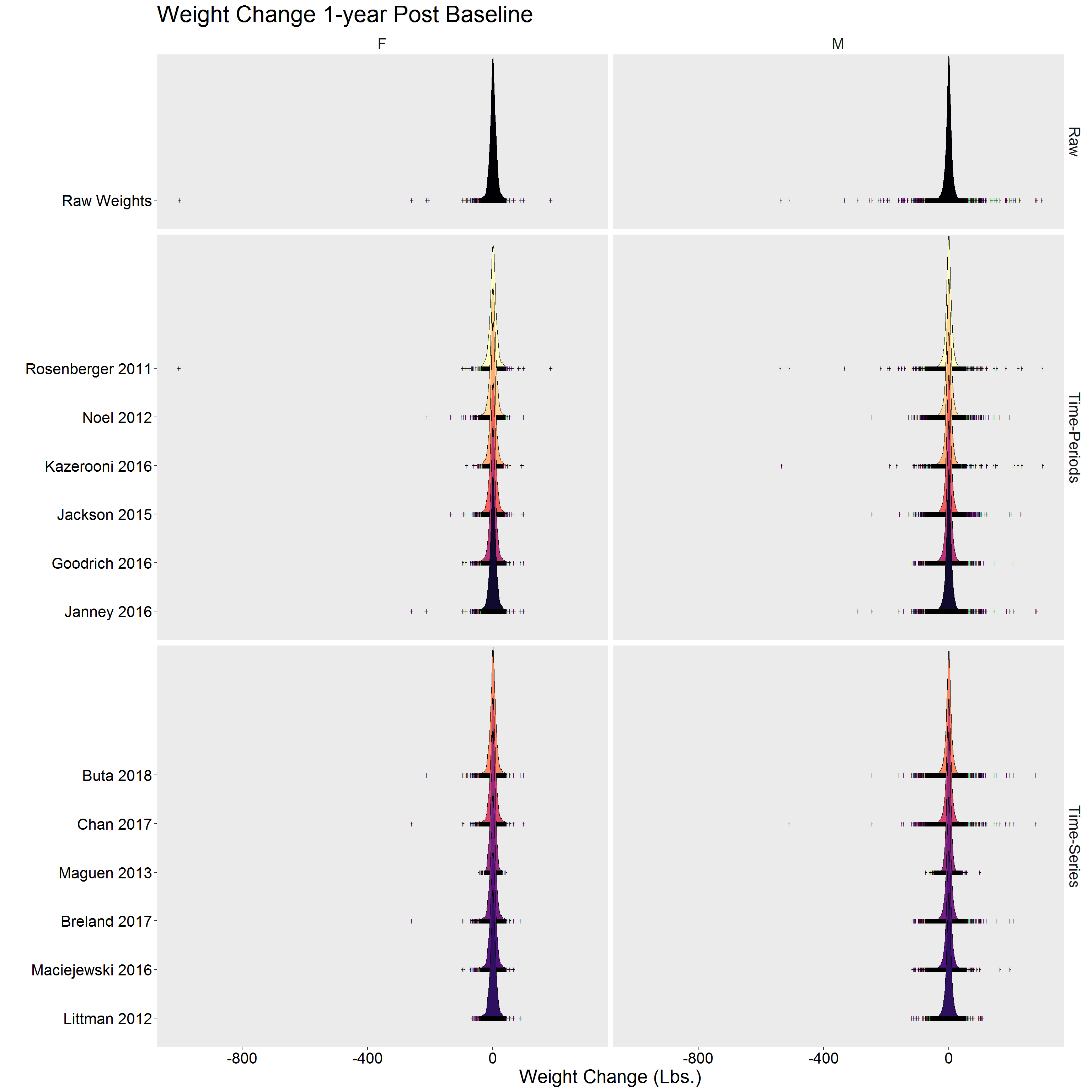

Alternative view

p <- DF %>%
  filter(!is.na(diff)) %>% 
  group_by(Algorithm) %>% 
  mutate(dens = approxfun(density(diff))(diff)) %>% 
  ggplot(aes(y = Algorithm, x = diff, color = dens)) %>% 
  add(geom_jitter(size = 2)) %>% 
  add(scale_color_viridis_c()) %>% 
  add(facet_grid(Type ~ Gender, scales = "free_y", space = "free_y")) %>%
  add(theme(
    legend.position = "none", 
    text = element_text(size = 20), 
    axis.text = element_text(color = "black"), 
    panel.grid = element_blank(), 
    strip.background = element_blank()
  )) %>%
  add(labs(
      x = "Weight Change (Lbs.)", 
      y = "",
      title = ""
  ))

p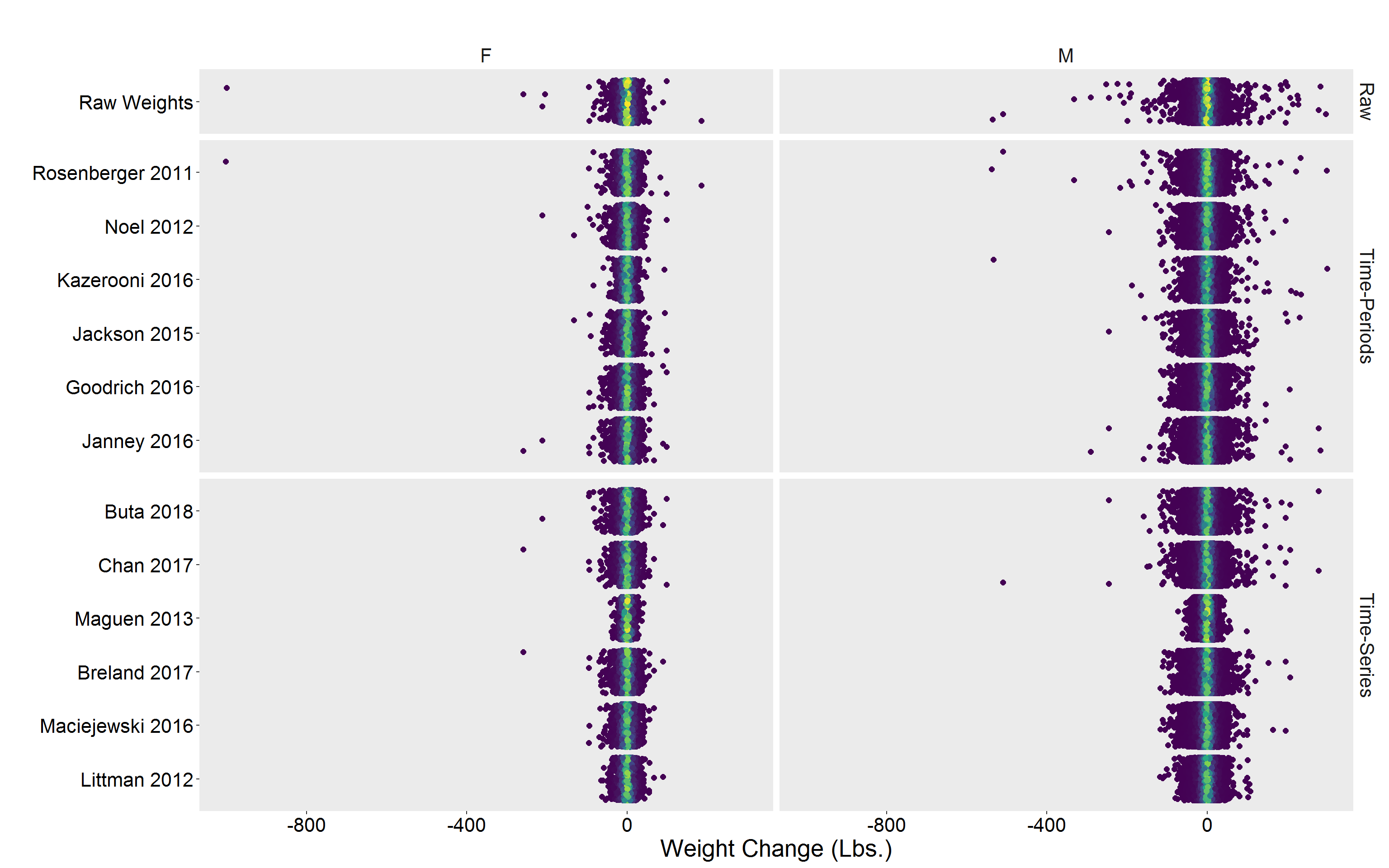

Site/Facility Level Analyses

Sta3n_wtdx_diff <- DF %>%
  select(Algorithm, Gender, Sta3n, diff, diff_perc) %>%
  reshape2::melt(id.vars = c("Gender", "Algorithm", "Sta3n")) %>%
  group_by(Gender, Algorithm, Sta3n, variable) %>%
  na.omit() %>%
  summarize(
    n      = n(),
    mean   = mean(value),
    median = median(value)
  ) %>%
  pivot_wider(
    names_from = variable,
    values_from = c("n", "mean", "median")
  )

Sta3n_wtpct <- DF %>%
  select(Gender, Algorithm, Sta3n, contains("weight")) %>%
  reshape2::melt(id.vars = c("Gender", "Algorithm", "Sta3n")) %>%
  group_by(Gender, Algorithm, Sta3n, variable) %>% 
  summarize(prop = sum(value == 1) / n()) %>% 
  pivot_wider(names_from = variable, values_from = "prop")

Sta3n_wtdx <- Sta3n_wtdx_diff %>%
  left_join(Sta3n_wtpct, by = c("Gender", "Algorithm", "Sta3n")) %>%
  left_join(
    DF %>%
      distinct(Algorithm, Type),
    by = "Algorithm"
  ) %>%
  select(
    Type,
    Gender,
    Sta3n,
    n_diff,
    mean_diff,
    median_diff,
    mean_diff_perc,
    median_diff_perc,
    gt5perc_weightloss,
    gt5perc_weightgain
  ) %>%
  ungroup()

rm(Sta3n_wtdx_diff, Sta3n_wtpct)

COLS <- c("#2E364F", "#2D5D7C", "#F3F0E2", "#EF5939")

p <- Sta3n_wtdx %>%
  ggplot(aes(mean_diff, group = Gender, fill = Gender)) %>%
  add(geom_histogram(bins = 100, alpha = 0.5)) %>%
  add(theme_minimal(16)) %>%
  add(theme(legend.position = c(0.2, 0.8))) %>%
  add(scale_fill_manual(values = COLS[c(2, 4)])) %>%
  add(labs(
    x = "Weight Change (lbs.)",
    y = "Frequency",
    fill = ""
  ))

q <- Sta3n_wtdx %>%
  filter(!is.infinite(mean_diff_perc)) %>%
  ggplot(aes(mean_diff_perc, group = Gender, fill = Gender)) %>%
  add(geom_histogram(bins = 100, alpha = 0.5)) %>%
  add(theme_minimal(16)) %>%
  add(theme(legend.position = "none")) %>%
  add(scale_fill_manual(values = COLS[c(2, 4)])) %>%
  add(labs(
    x = "Weight Change %",
    y = "Frequency",
    fill = ""
  ))

r <- Sta3n_wtdx %>%
  ggplot(aes(gt5perc_weightloss, group = Gender, fill = Gender)) %>%
  add(geom_histogram(bins = 100, alpha = 0.5)) %>%
  add(theme_minimal(16)) %>%
  add(theme(legend.position = "none")) %>%
  add(scale_fill_manual(values = COLS[c(2, 4)])) %>%
  add(labs(
    x = ">= 5% Weight Loss",
    y = "Frequency"
  ))

s <- Sta3n_wtdx %>%
  filter(!is.na(gt5perc_weightgain)) %>%
  ggplot(aes(gt5perc_weightgain, group = Gender, fill = Gender)) %>%
  add(geom_histogram(bins = 100, alpha = 0.5)) %>%
  add(theme_minimal(16)) %>%
  add(theme(legend.position = "none")) %>%
  add(scale_fill_manual(values = COLS[c(2, 4)])) %>%
  add(labs(
    x = ">= 5% Weight Gain",
    y = "Frequency"
  ))

library(patchwork)

p + q + r + s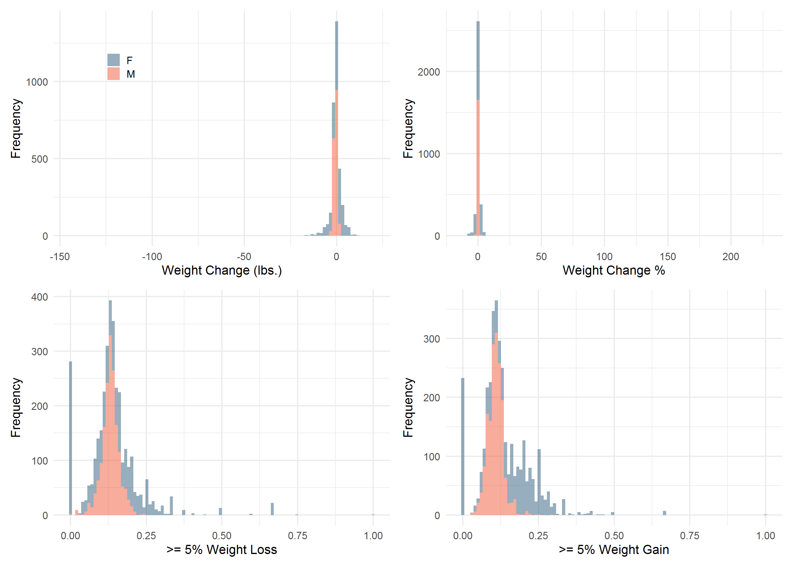

library(gridExtra)

tmp <- Sta3n_wtdx %>%
  select(Gender, Type, Algorithm, Sta3n, gt5perc_weightloss)

raw <- tmp %>% 
  filter(Algorithm == "Raw Weights") %>% 
  group_by(Gender) %>%
  arrange(gt5perc_weightloss) %>%
  mutate(Sta3n_rank = row_number()) %>%
  select(-Type, -Algorithm) %>%
  rename(raw_wtloss = gt5perc_weightloss)

tp <- tmp %>%
  filter(Type == "Time-Periods") %>%
  left_join(raw, by = c("Sta3n", "Gender")) %>%
  mutate(loss_diff = gt5perc_weightloss - raw_wtloss)
  
ts <- tmp %>%
  filter(Type == "Time-Series") %>%
  left_join(raw, by = c("Sta3n", "Gender")) %>%
  mutate(loss_diff = gt5perc_weightloss - raw_wtloss)

p1 <- tp %>%
  ggplot(aes(x = Sta3n_rank, y = raw_wtloss)) %>%
  add(facet_wrap(vars(Type, Gender))) %>%
  add(geom_line(size = 1)) %>%
  add(geom_segment(
    aes(
      x = Sta3n_rank,
      y = raw_wtloss,
      xend = Sta3n_rank,
      yend = gt5perc_weightloss
    ),
    alpha = 0.3
  )) %>%
  add(geom_point(
    aes(
      x = Sta3n_rank, 
      y = gt5perc_weightloss, 
      color = Algorithm
    ),
    size = 2,
    alpha = 0.7
  )) %>%
  add(expand_limits(y = c(0.0, 0.3))) %>%
  add(theme_minimal(16)) %>%
  add(theme(
    legend.position = "bottom",
    panel.grid.major.x = element_blank(),
    panel.grid.minor.x = element_blank()
  )) %>%
  add(guides(color = guide_legend(override.aes = list(size = 5)))) %>%
  add(scale_color_brewer(palette = "Dark2")) %>%
  add(labs(
    x = "Sta3n",
    y = "Proportion Achieving 5% Weight Loss",
    color = ""
  ))

p2 <- p1 %+% ts
p2 <- p2 %>% add(labs(y = ""))
grid.arrange(p1, p2, ncol = 2)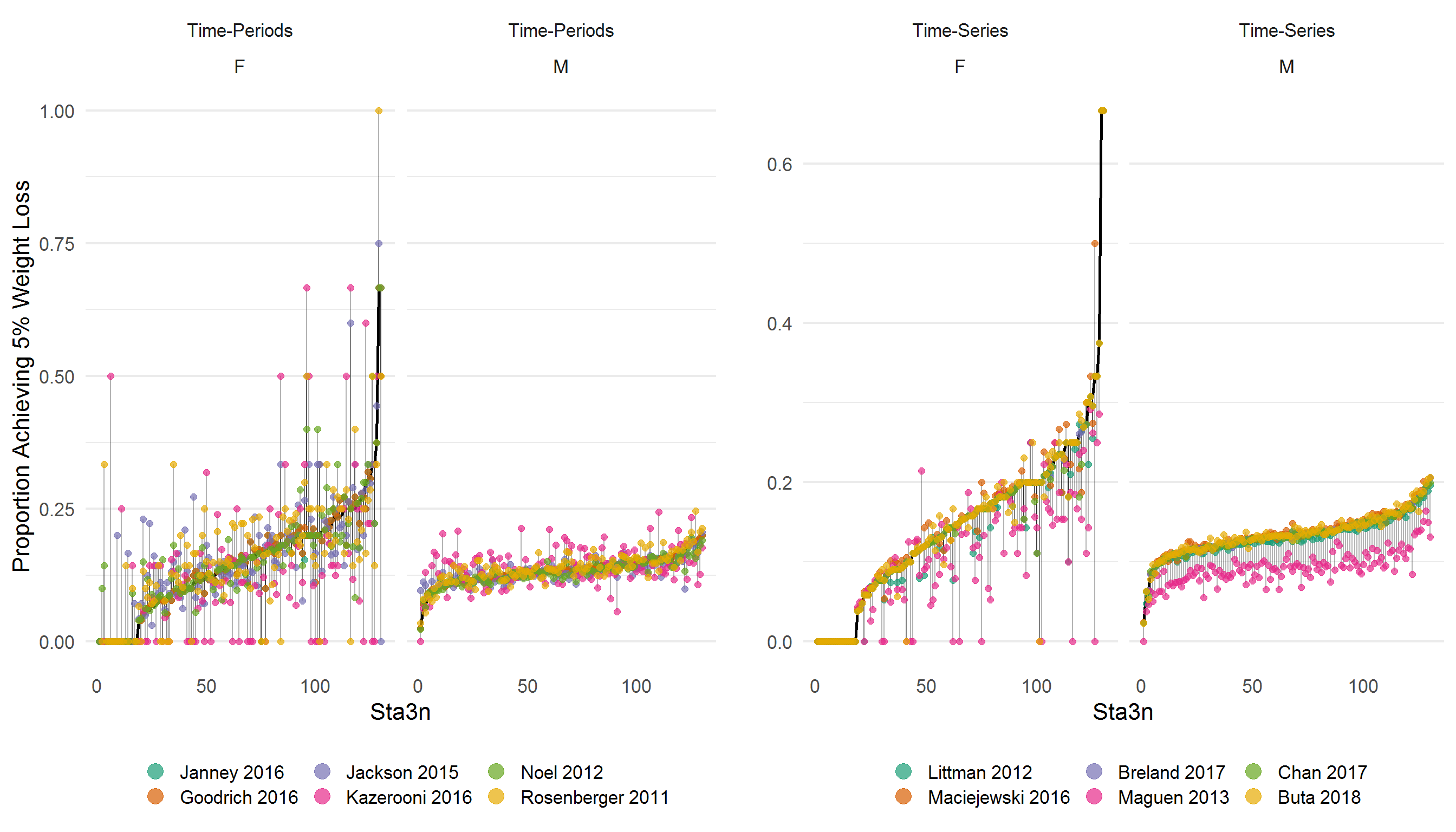

Sites are ordered/ranked along the x-axis using the percent of patients with at least 5% weight loss using the raw data. The left hand side shows the “time-period” algorithms, while the right displays the “time-series” algorithms. Results suggest that generally, time-series algorithms may result in more similar rates by site, save for Maguen 2013. Results are more mixed using the “time-period” algorithms.

By BMI Category

BMI works differently for Men and Women, so I’ll use only the Males for this analysis.

Total number of weight samples, by BMI category

bmi_cohort <- weight.ls[[2]] %>%
  filter(Gender == "M", !is.na(BMI)) %>%
  group_by(PatientICN) %>%
  arrange(PatientICN, WeightDateTime) %>%
  filter(row_number() == 1) %>%
  mutate(
    BMI_cat = case_when(
      BMI < 18.5               ~ 0,
      BMI >= 18.5 & BMI < 24.9 ~ 1,
      BMI >= 24.9 & BMI < 30   ~ 2,
      BMI >= 30                ~ 3
    ),
    BMI_cat = factor(
      BMI_cat,
      0:3,
      c("Underweight", "Normal", "Overweight", "Obese")
    )
  ) %>%
  select(PatientICN, BMI_cat) %>%
  left_join(weight.ls[[2]], by = "PatientICN") %>%
  relocate(BMI_cat, .after = last_col()) %>%
  ungroup()

bmi_cohort %>%
  janitor::tabyl(BMI_cat) %>%
  arrange(desc(n)) %>%
  adorn_pct_formatting() %>%
  tableStyle()

BMI_cat	n	percent
Obese	505717	47.8%
Overweight	371623	35.1%
Normal	171864	16.2%
Underweight	9174	0.9%

Total number of people

bmi_cohort %>%
  distinct(PatientICN, BMI_cat) %>%
  tabyl(BMI_cat) %>%
  adorn_pct_formatting() %>%
  tableStyle()

BMI_cat	n	percent
Underweight	629	0.7%
Normal	14662	16.9%
Overweight	33243	38.4%
Obese	38103	44.0%

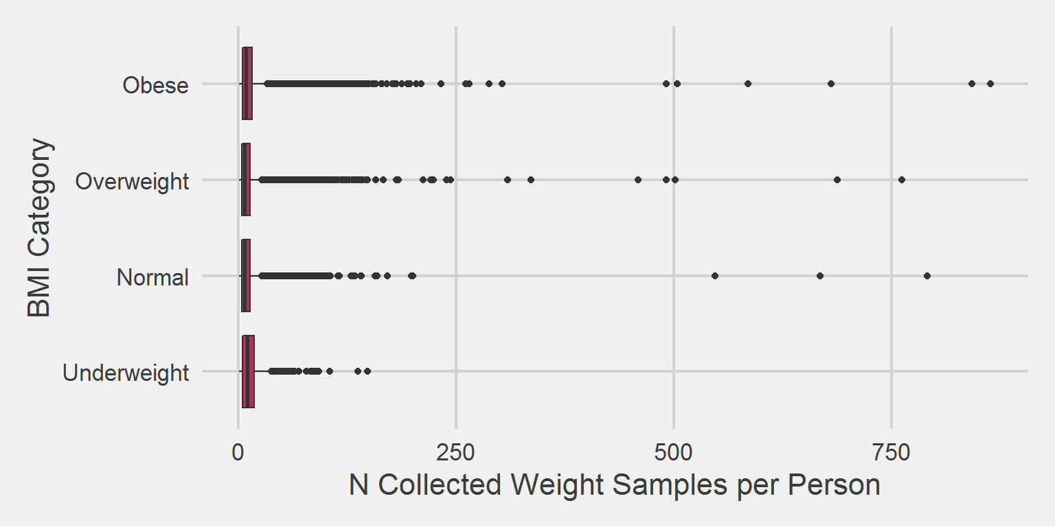
Association between number of weight samples collected, and BMI category,

bmi_cohort %>%
  group_by(BMI_cat) %>%
  count(PatientICN) %>%
  summarise(
    mean   = mean(n),
    SD     = sd(n),
    median = median(n),
    min    = min(n),
    max    = max(n)
  ) %>%
  tableStyle()

BMI_cat	mean	SD	median	min	max
Underweight	14.59	16.35	10	1	148
Normal	11.72	26.84	7	1	1525
Overweight	11.18	16.93	7	1	1254
Obese	13.27	18.36	9	1	1196

bmi_cohort %>%
  group_by(BMI_cat) %>%
  count(PatientICN) %>%
  filter(n < 1000) %>%
  ggplot(aes(x = BMI_cat, y = n)) %>%
  add(geom_boxplot(fill = "maroon")) %>%
  add(theme_fivethirtyeight(16)) %>%
  add(theme(axis.title = element_text())) %>%
  add(coord_flip()) %>%
  add(labs(
    x = "BMI Category",
    y = "N Collected Weight Samples per Person"
  ))

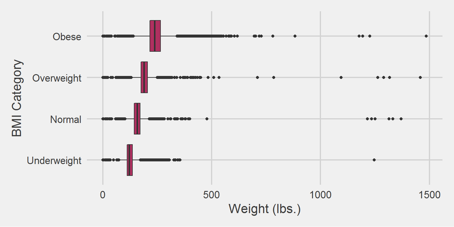
All weight in lbs. by BMI category, for the 2016 cohort only

bmi_cohort %>%
  group_by(BMI_cat) %>%
  summarise(
    mean   = mean(Weight),
    SD     = sd(Weight),
    median = median(Weight),
    min    = min(Weight),
    max    = max(Weight)
  ) %>%
  tableStyle()

BMI_cat	mean	SD	median	min	max
Underweight	126.11	29.42	121.0	0	1246.00
Normal	157.37	22.39	156.7	0	1370.04
Overweight	189.66	23.60	189.0	0	1458.15
Obese	243.42	42.90	236.6	0	1486.20

It would also make sense to look at this from the perspective of BMI ranges,

bmi_cohort %>%
  group_by(BMI_cat) %>%
  summarise(
    mean   = mean(BMI),
    SD     = sd(BMI),
    median = median(BMI),
    min    = min(BMI),
    max    = max(BMI)
  ) %>%
  tableStyle()

BMI_cat	mean	SD	median	min	max
Underweight	18.15	3.96	17.62	0	178.76
Normal	22.80	2.62	22.96	0	227.96
Overweight	27.40	2.49	27.44	0	215.31
Obese	35.15	8.32	33.98	0	1525.51

It’s illuminating in the context of outliers, but we already know this from analyzing the weight samples themselves.

bmi_cohort %>%
  ggplot(aes(x = BMI_cat, y = Weight)) %>%
  add(geom_boxplot(fill = "maroon")) %>%
  add(theme_fivethirtyeight(16)) %>%
  add(theme(axis.title = element_text())) %>%
  add(coord_flip()) %>%
  add(labs(
    x = "BMI Category",
    y = "Weight (lbs.)"
  ))

By Algorithm

raw <- bmi_cohort %>%
  select(PatientICN, Weight, BMI_cat)

#---- apply Janney et al. 2016 ----#

Janney2016.df <- Janney2016.f(
  DF = bmi_cohort,
  id = "PatientICN",
  measures = "Weight",
  tmeasures = "WeightDateTime",
  startPoint = "VisitDateTime"
) %>%
  select(PatientICN, Weight_OR, BMI_cat) %>%
  rename(Weight = Weight_OR) %>%
  na.omit()

#---- apply Littman et al. 2012 ----#

Littman2012.df <- Littman2012.f(
  DF = bmi_cohort,
  id = "PatientICN",
  measures = "Weight",
  tmeasures = "WeightDateTime"
) %>%
  select(PatientICN, OutputMeasurement, BMI_cat) %>%
  rename(Weight = OutputMeasurement) %>%
  na.omit()

#---- Coerce Maciejewski et al. 2016 to a workable format ----#

Maciejewski2016.df <- maciejewski %>%
  filter(IO == "Output", SampleYear == "2016") %>%
  mutate(PatientICN = as.character(PatientICN)) %>%
  left_join(
    raw %>%
      distinct(PatientICN, BMI_cat),
    by = "PatientICN"
  ) %>%
  select(PatientICN, Weight, BMI_cat) %>%
  na.omit()

#---- Apply Breland et al. 2017 ----#

Breland2017.df <- Breland2017.f(
  DF = bmi_cohort,
  id = "PatientICN",
  measures = "Weight",
  tmeasures = "WeightDateTime"
) %>%
  select(PatientICN, measures_aug_, BMI_cat) %>%
  rename(Weight = measures_aug_) %>%
  na.omit()

#---- Apply Maguen et al. 2013 ----#

Maguen2013.df <- Maguen2013.f(
  DF = bmi_cohort,
  id = "PatientICN",
  measures = "Weight",
  tmeasures = "WeightDateTime",
  variables = "AgeAtVisit"
) %>%
  select(PatientICN, Output, BMI_cat) %>%
  rename(Weight = Output) %>%
  na.omit()

#---- Apply Goodrich 2016 ----#

Goodrich2016.df <- Goodrich2016.f(
  DF = bmi_cohort,
  id = "PatientICN",
  measures = "Weight",
  tmeasures = "WeightDateTime",
  startPoint = "VisitDateTime"
) %>%
  select(PatientICN, output, BMI_cat) %>%
  rename(Weight = output) %>%
  na.omit()

#---- Apply Chan & Raffa 2017 ----#

Chan2017.df <- Chan2017.f(
  DF = bmi_cohort,
  id = "PatientICN",
  measures = "Weight",
  tmeasures = "WeightDateTime"
) %>%
  select(PatientICN, measures_aug_, BMI_cat) %>%
  rename(Weight = measures_aug_) %>%
  na.omit()

#---- Apply Jackson et al. 2015 ----#

Jackson2015.df <- Jackson2015.f(
  DF = bmi_cohort,
  id = "PatientICN",
  measures = "Weight",
  tmeasures = "WeightDateTime",
  startPoint = "VisitDateTime"
) %>%
  left_join(
    bmi_cohort %>%
      distinct(PatientICN, BMI_cat),
    by = "PatientICN"
  ) %>%
  select(PatientICN, BMI_cat, output) %>%
  rename(Weight = output) %>%
  na.omit()

#---- Apply Buta et al., 2018 ----#

Buta2018.df <- Buta2018.f(
  DF = bmi_cohort,
  id = "PatientICN",
  measures = "BMI",
  tmeasures = "WeightDateTime"
) %>%
  select(PatientICN, BMI_cat, Weight) %>%
  na.omit()

#---- Apply Kazerooni & Lim, 2016 ----#

Kazerooni2016.df <- Kazerooni2016.f(
  DF = bmi_cohort,
  id = "PatientICN",
  measures = "Weight",
  tmeasures = "WeightDateTime",
  startPoint = "VisitDateTime"
) %>%
  select(PatientICN, BMI_cat, Weight) %>%
  na.omit()

#---- Apply Noel et al., 2012 ----#

Noel2012.df <- Noel2012.f(
  DF = bmi_cohort,
  id = "PatientICN",
  measures = "Weight",
  tmeasures = "WeightDateTime"
) %>% 
  distinct(PatientICN, BMI_cat, FYQ, Qmedian) %>%
  select(-FYQ) %>%
  rename(Weight = Qmedian) %>%
  na.omit()

#---- Apply Rosenberger et al., 2011 ----#

Rosenberger2011.df <- Rosenberger2011.f(
  DF = bmi_cohort,
  id = "PatientICN",
  tmeasures = "WeightDateTime",
  startPoint = "VisitDateTime",
  pad = 1
) %>%
  select(PatientICN, BMI_cat, Weight) %>%
  na.omit()

# stack original (raw), janney 2016, littman 2012, maciejewski 2016, 
# Breland 2017, Maguen 2013, Goodrich 2016, Chan & Raffa 2017, 
# Jackson 2015, Buta 2018, Kazerooni & Lim 2016, Noel 2012,
# and Rosenberger 2011 processed weights
  
algos.fac  <- c("Raw Weights",
                "Janney 2016",
                "Littman 2012",
                "Maciejewski 2016",
                "Breland 2017",
                "Maguen 2013",
                "Goodrich 2016",
                "Chan 2017",
                "Jackson 2015",
                "Buta 2018",
                "Kazerooni 2016",
                "Noel 2012",
                "Rosenberger 2011")

DF <- bind_rows(
  list(`Raw Weights`      = raw,
       `Janney 2016`      = Janney2016.df,
       `Littman 2012`     = Littman2012.df,
       `Maciejewski 2016` = Maciejewski2016.df,
       `Breland 2017`     = Breland2017.df,
       `Maguen 2013`      = Maguen2013.df,
       `Goodrich 2016`    = Goodrich2016.df,
       `Chan 2017`        = Chan2017.df,
       `Jackson 2015`     = Jackson2015.df,
       `Buta 2018`        = Buta2018.df,
       `Kazerooni 2016`   = Kazerooni2016.df,
       `Noel 2012`        = Noel2012.df,
       `Rosenberger 2011` = Rosenberger2011.df),
  .id = "Algorithm"
)

rm(
  Buta2018.df,
  Kazerooni2016.df,
  Noel2012.df,
  Rosenberger2011.df,
  Breland2017.df,
  Chan2017.df,
  Goodrich2016.df,
  Jackson2015.df,
  Janney2016.df,
  Littman2012.df,
  Maciejewski2016.df,
  Maguen2013.df,
  raw
)

DF$Algorithm <- factor(DF$Algorithm, levels = algos.fac, labels = algos.fac)

DF$Type <- case_when(
  DF$Algorithm == "Raw Weights"                  ~ 1,
  DF$Algorithm %in% algos.fac[c(2, 7, 9, 11:13)] ~ 2,
  DF$Algorithm %in% algos.fac[c(3:6, 8, 10)]     ~ 3
)
DF$Type <- factor(DF$Type, 1:3, c("Raw", "Time-Periods", "Time-Series"))

Total weight measurements, by algorithm and Sex.

DF %>%
  tabyl(Algorithm, BMI_cat) %>%
  adorn_percentages() %>%
  adorn_pct_formatting() %>%
  adorn_ns() %>%
  tableStyle()

Algorithm	Underweight	Normal	Overweight	Obese
Raw Weights	0.9% (9174)	16.2% (171864)	35.1% (371623)	47.8% (505717)
Janney 2016	0.7% (1256)	16.2% (28727)	37.9% (67155)	45.1% (79837)
Littman 2012	0.9% (8915)	16.2% (169459)	35.2% (367844)	47.8% (499858)
Maciejewski 2016	0.9% (8838)	16.0% (164857)	35.2% (362454)	47.9% (492648)
Breland 2017	0.9% (9135)	16.2% (171726)	35.1% (371437)	47.8% (505338)
Maguen 2013	0.9% (8339)	17.0% (158002)	36.3% (338323)	45.8% (426941)
Goodrich 2016	0.7% (1265)	16.2% (28713)	37.9% (67136)	45.1% (79818)
Chan 2017	0.9% (9103)	16.2% (170995)	35.1% (369876)	47.8% (503380)
Jackson 2015	0.7% (1538)	16.1% (35908)	37.8% (84435)	45.4% (101254)
Buta 2018	0.9% (9113)	16.2% (171333)	35.1% (370629)	47.8% (504637)
Kazerooni 2016	0.9% (576)	15.3% (9909)	35.4% (22992)	48.4% (31461)
Noel 2012	0.7% (4411)	15.9% (96637)	36.9% (224645)	46.5% (282526)
Rosenberger 2011	0.7% (1336)	15.4% (31400)	37.2% (75674)	46.8% (95247)

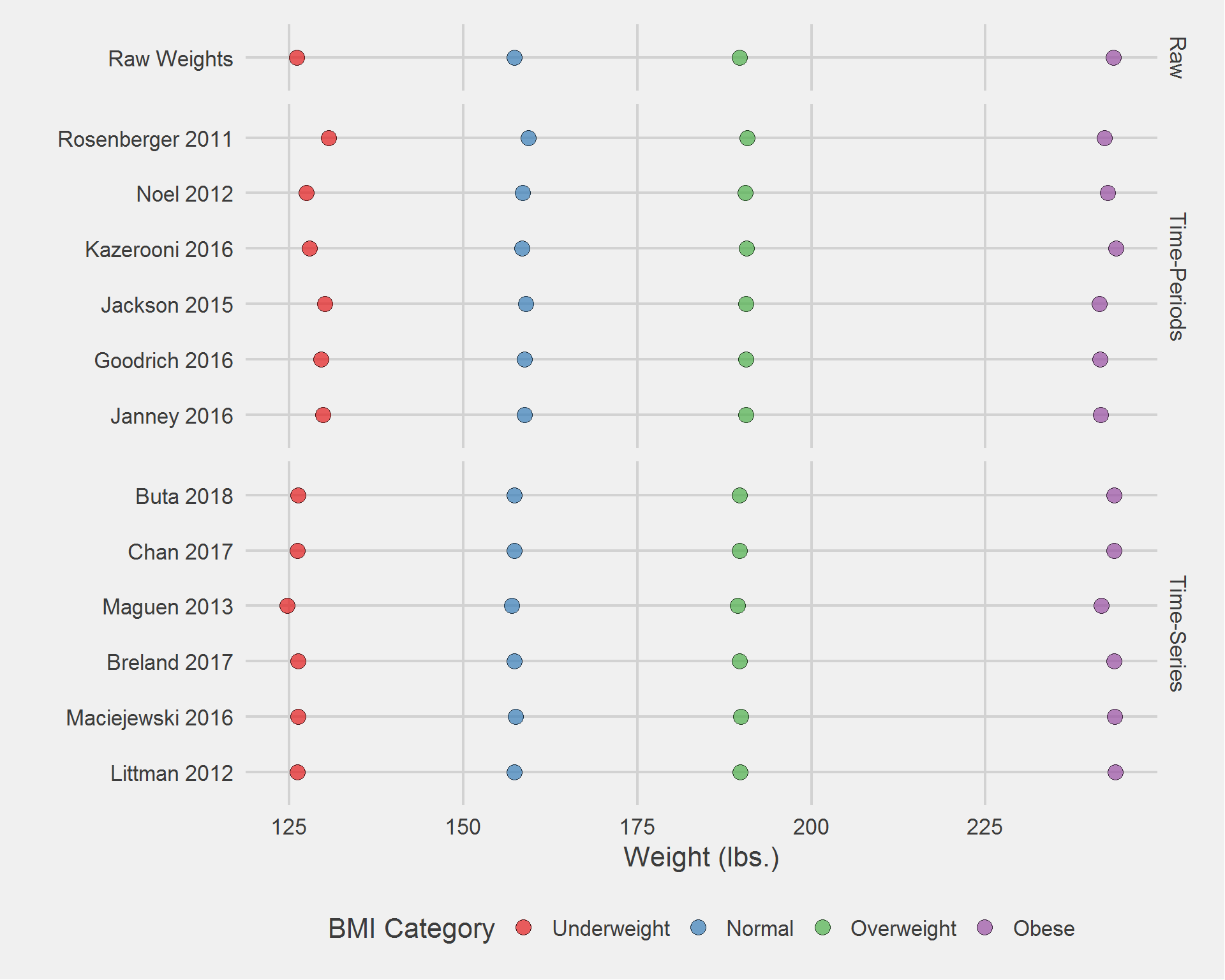
Distribution of weight measurements, by algorithm and BMI category

tmp <- DF %>%
  filter(!is.na(Weight)) %>%
  group_by(Type, Algorithm, BMI_cat) %>%
  dplyr::summarise(
    weight_n = n(),
    mean     = mean(Weight),
    SD       = sd(Weight),
    median   = median(Weight),
    IQR      = IQR(Weight),
    min      = min(Weight),
    max      = max(Weight)
  )


tableStyle(tmp)

Type	Algorithm	BMI_cat	weight_n	mean	SD	median	IQR	min	max
Raw	Raw Weights	Underweight	9174	126.11	29.42	121.00	24.50	0.00	1246.00
Raw	Raw Weights	Normal	171864	157.37	22.39	156.70	28.00	0.00	1370.04
Raw	Raw Weights	Overweight	371623	189.66	23.60	189.00	30.00	0.00	1458.15
Raw	Raw Weights	Obese	505717	243.42	42.90	236.60	50.00	0.00	1486.20
Time-Periods	Janney 2016	Underweight	1256	129.92	32.02	123.00	25.03	82.60	351.60
Time-Periods	Janney 2016	Normal	28727	158.83	20.73	158.10	27.00	80.00	478.00
Time-Periods	Janney 2016	Overweight	67155	190.59	22.19	190.00	29.40	92.20	533.30
Time-Periods	Janney 2016	Obese	79837	241.51	40.08	235.10	47.80	98.40	546.00
Time-Periods	Goodrich 2016	Underweight	1265	129.59	32.13	123.00	25.40	80.20	351.60
Time-Periods	Goodrich 2016	Normal	28713	158.82	20.68	158.00	27.00	80.00	478.00
Time-Periods	Goodrich 2016	Overweight	67136	190.58	22.12	190.00	29.40	96.00	368.17
Time-Periods	Goodrich 2016	Obese	79818	241.49	40.01	235.10	47.80	87.00	500.00
Time-Periods	Jackson 2015	Underweight	1538	130.19	33.51	123.00	25.61	78.00	354.50
Time-Periods	Jackson 2015	Normal	35908	158.96	20.90	158.30	27.05	83.38	365.97
Time-Periods	Jackson 2015	Overweight	84435	190.57	22.46	189.80	29.73	95.30	449.74
Time-Periods	Jackson 2015	Obese	101254	241.36	40.25	235.00	48.00	87.00	553.00
Time-Periods	Kazerooni 2016	Underweight	576	127.98	32.19	121.00	26.35	82.50	342.80
Time-Periods	Kazerooni 2016	Normal	9909	158.46	24.09	157.90	28.00	16.50	1233.70
Time-Periods	Kazerooni 2016	Overweight	22992	190.71	23.25	189.90	30.25	16.50	710.00
Time-Periods	Kazerooni 2016	Obese	31461	243.75	41.66	237.20	49.90	0.00	517.44
Time-Periods	Noel 2012	Underweight	4411	127.49	28.53	122.15	23.30	70.00	354.50
Time-Periods	Noel 2012	Normal	96637	158.55	20.30	158.00	26.50	74.00	365.97
Time-Periods	Noel 2012	Overweight	224645	190.53	21.90	189.80	28.90	70.00	449.74
Time-Periods	Noel 2012	Obese	282526	242.52	40.40	236.00	48.00	71.25	588.90
Time-Periods	Rosenberger 2011	Underweight	1336	130.68	34.40	123.50	26.00	22.90	354.50
Time-Periods	Rosenberger 2011	Normal	31400	159.34	22.17	159.00	27.80	11.02	1314.50
Time-Periods	Rosenberger 2011	Overweight	75674	190.76	22.99	190.00	29.90	1.00	710.00
Time-Periods	Rosenberger 2011	Obese	95247	242.09	40.83	235.80	48.49	0.00	727.50
Time-Series	Littman 2012	Underweight	8915	126.17	26.27	121.00	24.10	75.20	354.50
Time-Series	Littman 2012	Normal	169459	157.33	20.84	156.70	28.00	75.30	365.97
Time-Series	Littman 2012	Overweight	367844	189.74	22.82	189.00	29.80	78.00	356.00
Time-Series	Littman 2012	Obese	499858	243.61	42.36	236.80	50.00	88.00	546.00
Time-Series	Maciejewski 2016	Underweight	8838	126.31	26.54	121.10	24.20	66.00	354.50
Time-Series	Maciejewski 2016	Normal	164857	157.53	21.03	156.97	28.00	64.00	365.97
Time-Series	Maciejewski 2016	Overweight	362454	189.84	22.78	189.00	29.89	87.00	318.00
Time-Series	Maciejewski 2016	Obese	492648	243.58	42.46	236.90	50.00	93.00	546.00
Time-Series	Breland 2017	Underweight	9135	126.26	26.45	121.03	24.25	75.20	354.50
Time-Series	Breland 2017	Normal	171726	157.35	21.12	156.70	28.00	77.00	365.97
Time-Series	Breland 2017	Overweight	371437	189.67	23.00	189.00	30.00	82.50	379.20
Time-Series	Breland 2017	Obese	505338	243.48	42.56	236.60	50.00	93.00	694.46
Time-Series	Maguen 2013	Underweight	8339	124.71	24.05	120.50	23.48	74.60	345.00
Time-Series	Maguen 2013	Normal	158002	157.00	20.24	156.31	27.38	74.00	343.10
Time-Series	Maguen 2013	Overweight	338323	189.44	22.16	188.80	29.20	95.70	309.00
Time-Series	Maguen 2013	Obese	426941	241.65	40.07	235.07	47.20	103.80	541.10
Time-Series	Chan 2017	Underweight	9103	126.20	26.54	121.00	24.40	64.00	354.50
Time-Series	Chan 2017	Normal	170995	157.34	21.13	156.70	28.00	58.60	365.97
Time-Series	Chan 2017	Overweight	369876	189.67	22.99	189.00	30.00	59.00	509.27
Time-Series	Chan 2017	Obese	503380	243.49	42.57	236.60	50.00	54.00	727.50
Time-Series	Buta 2018	Underweight	9113	126.29	26.52	121.04	24.20	66.80	354.50
Time-Series	Buta 2018	Normal	171333	157.38	21.26	156.70	28.00	67.46	478.00
Time-Series	Buta 2018	Overweight	370629	189.67	23.09	189.00	30.00	74.50	509.27
Time-Series	Buta 2018	Obese	504637	243.42	42.55	236.60	50.00	66.50	540.00

tmp %>%
  ggplot(aes(mean, Algorithm)) %>%
  add(geom_point(aes(fill = BMI_cat), size = 4, pch = 21, alpha = 0.7)) %>%
  add(facet_grid(rows = vars(Type), scales = "free", space = "free")) %>%
  add(theme_fivethirtyeight(16)) %>%
  add(theme(axis.title = element_text())) %>%
  add(scale_fill_brewer(palette = "Set1")) %>%
  add(labs(
    x = "Weight (lbs.)",
    y = "",
    fill = "BMI Category"
  ))

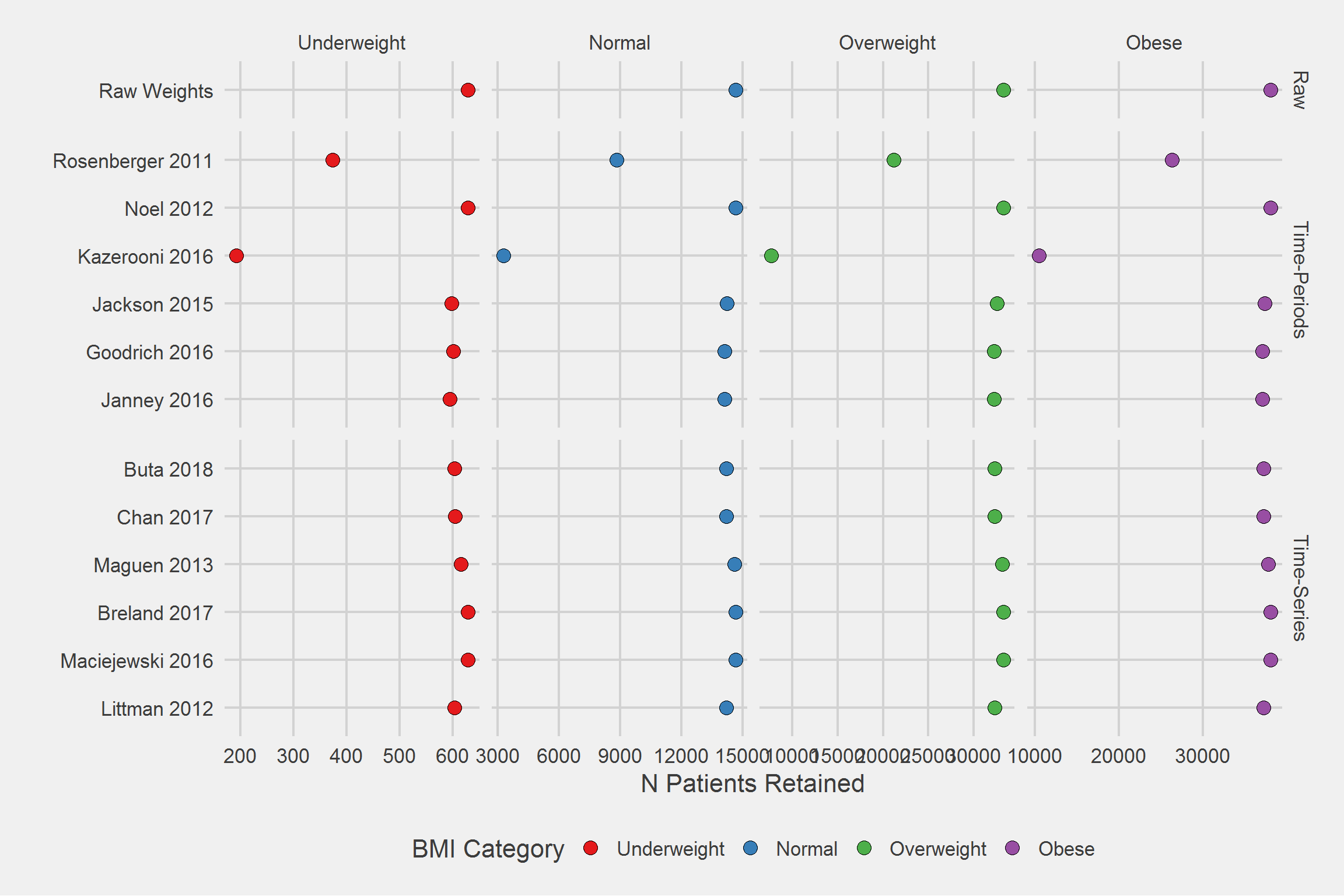
Number of Patients/Veterans Retained, by algorithm, by BMI category

tmp <- DF %>%
  filter(!is.na(Weight)) %>%
  group_by(Type, Algorithm, BMI_cat) %>%
  distinct(PatientICN) %>%
  count()

tableStyle(tmp)

Type	Algorithm	BMI_cat	n
Raw	Raw Weights	Underweight	629
Raw	Raw Weights	Normal	14662
Raw	Raw Weights	Overweight	33243
Raw	Raw Weights	Obese	38103
Time-Periods	Janney 2016	Underweight	595
Time-Periods	Janney 2016	Normal	14116
Time-Periods	Janney 2016	Overweight	32250
Time-Periods	Janney 2016	Obese	37102
Time-Periods	Goodrich 2016	Underweight	601
Time-Periods	Goodrich 2016	Normal	14117
Time-Periods	Goodrich 2016	Overweight	32247
Time-Periods	Goodrich 2016	Obese	37100
Time-Periods	Jackson 2015	Underweight	598
Time-Periods	Jackson 2015	Normal	14235
Time-Periods	Jackson 2015	Overweight	32533
Time-Periods	Jackson 2015	Obese	37395
Time-Periods	Kazerooni 2016	Underweight	192
Time-Periods	Kazerooni 2016	Normal	3303
Time-Periods	Kazerooni 2016	Overweight	7664
Time-Periods	Kazerooni 2016	Obese	10487
Time-Periods	Noel 2012	Underweight	629
Time-Periods	Noel 2012	Normal	14662
Time-Periods	Noel 2012	Overweight	33243
Time-Periods	Noel 2012	Obese	38103
Time-Periods	Rosenberger 2011	Underweight	374
Time-Periods	Rosenberger 2011	Normal	8839
Time-Periods	Rosenberger 2011	Overweight	21208
Time-Periods	Rosenberger 2011	Obese	26324
Time-Series	Littman 2012	Underweight	604
Time-Series	Littman 2012	Normal	14201
Time-Series	Littman 2012	Overweight	32339
Time-Series	Littman 2012	Obese	37280
Time-Series	Maciejewski 2016	Underweight	629
Time-Series	Maciejewski 2016	Normal	14662
Time-Series	Maciejewski 2016	Overweight	33243
Time-Series	Maciejewski 2016	Obese	38103
Time-Series	Breland 2017	Underweight	629
Time-Series	Breland 2017	Normal	14662
Time-Series	Breland 2017	Overweight	33243
Time-Series	Breland 2017	Obese	38103
Time-Series	Maguen 2013	Underweight	616
Time-Series	Maguen 2013	Normal	14604
Time-Series	Maguen 2013	Overweight	33128
Time-Series	Maguen 2013	Obese	37781
Time-Series	Chan 2017	Underweight	605
Time-Series	Chan 2017	Normal	14201
Time-Series	Chan 2017	Overweight	32339
Time-Series	Chan 2017	Obese	37280
Time-Series	Buta 2018	Underweight	603
Time-Series	Buta 2018	Normal	14201
Time-Series	Buta 2018	Overweight	32339
Time-Series	Buta 2018	Obese	37267

tmp %>%
  ggplot(aes(x = Algorithm, y = n)) %>%
  add(geom_point(aes(fill = BMI_cat), size = 4, pch = 21)) %>%
  add(facet_grid(
    cols = vars(BMI_cat), 
    rows = vars(Type), 
    scales = "free",
    space = "free_y"
  )) %>%
  add(theme_fivethirtyeight(16)) %>%
  add(theme(axis.title = element_text())) %>%
  add(scale_fill_brewer(palette = "Set1")) %>%
  add(coord_flip()) %>%
  add(labs(
    x = "",
    y = "N Patients Retained",
    fill = "BMI Category"
  ))

Number of weights retained, per person, by algorithm, by BMI Category,

tmp <- DF %>%
  filter(!is.na(Weight)) %>%
  group_by(Type, Algorithm, BMI_cat, PatientICN) %>%
  count() %>%
  ungroup() %>%
  group_by(Type, Algorithm, BMI_cat) %>%
  summarize(
    mean   = mean(n),
    SD     = sd(n),
    min    = min(n),
    Q1     = fivenum(n)[2],
    median = median(n),
    Q3     = fivenum(n)[4],
    max    = max(n)
  )

tableStyle(tmp)

Type	Algorithm	BMI_cat	mean	SD	min	Q1	median	Q3	max
Raw	Raw Weights	Underweight	14.59	16.35	1	5	10	18.0	148
Raw	Raw Weights	Normal	11.72	26.84	1	4	7	13.0	1525
Raw	Raw Weights	Overweight	11.18	16.93	1	4	7	13.0	1254
Raw	Raw Weights	Obese	13.27	18.36	1	5	9	16.0	1196
Time-Periods	Janney 2016	Underweight	2.11	0.79	1	1	2	3.0	3
Time-Periods	Janney 2016	Normal	2.04	0.76	1	1	2	3.0	3
Time-Periods	Janney 2016	Overweight	2.08	0.75	1	2	2	3.0	3
Time-Periods	Janney 2016	Obese	2.15	0.76	1	2	2	3.0	3
Time-Periods	Goodrich 2016	Underweight	2.10	0.79	1	1	2	3.0	3
Time-Periods	Goodrich 2016	Normal	2.03	0.76	1	1	2	3.0	3
Time-Periods	Goodrich 2016	Overweight	2.08	0.75	1	2	2	3.0	3
Time-Periods	Goodrich 2016	Obese	2.15	0.76	1	2	2	3.0	3
Time-Periods	Jackson 2015	Underweight	2.57	1.01	1	2	3	3.0	4
Time-Periods	Jackson 2015	Normal	2.52	0.99	1	2	3	3.0	4
Time-Periods	Jackson 2015	Overweight	2.60	0.97	1	2	3	3.0	4
Time-Periods	Jackson 2015	Obese	2.71	0.98	1	2	3	3.0	4
Time-Periods	Kazerooni 2016	Underweight	3.00	0.00	3	3	3	3.0	3
Time-Periods	Kazerooni 2016	Normal	3.00	0.00	3	3	3	3.0	3
Time-Periods	Kazerooni 2016	Overweight	3.00	0.00	3	3	3	3.0	3
Time-Periods	Kazerooni 2016	Obese	3.00	0.00	3	3	3	3.0	3
Time-Periods	Noel 2012	Underweight	7.01	3.81	1	4	7	9.0	17
Time-Periods	Noel 2012	Normal	6.59	3.62	1	4	6	9.0	17
Time-Periods	Noel 2012	Overweight	6.76	3.63	1	4	6	9.0	17
Time-Periods	Noel 2012	Obese	7.41	3.81	1	4	7	10.0	17
Time-Periods	Rosenberger 2011	Underweight	3.57	0.50	3	3	4	4.0	4
Time-Periods	Rosenberger 2011	Normal	3.55	0.50	3	3	4	4.0	4
Time-Periods	Rosenberger 2011	Overweight	3.57	0.50	3	3	4	4.0	4
Time-Periods	Rosenberger 2011	Obese	3.62	0.49	3	3	4	4.0	4
Time-Series	Littman 2012	Underweight	14.76	16.16	2	5	10	18.0	148
Time-Series	Littman 2012	Normal	11.93	27.10	2	4	8	14.0	1524
Time-Series	Littman 2012	Overweight	11.37	16.97	2	4	8	13.0	1253
Time-Series	Littman 2012	Obese	13.41	18.31	2	5	9	16.0	1193
Time-Series	Maciejewski 2016	Underweight	14.05	15.39	1	5	10	17.0	139
Time-Series	Maciejewski 2016	Normal	11.24	17.29	1	4	7	13.0	629
Time-Series	Maciejewski 2016	Overweight	10.90	13.16	1	4	7	13.0	637
Time-Series	Maciejewski 2016	Obese	12.93	14.93	1	5	9	16.0	615
Time-Series	Breland 2017	Underweight	14.52	16.33	1	5	10	18.0	148
Time-Series	Breland 2017	Normal	11.71	26.79	1	4	7	13.0	1524
Time-Series	Breland 2017	Overweight	11.17	16.91	1	4	7	13.0	1251
Time-Series	Breland 2017	Obese	13.26	18.34	1	5	9	16.0	1192
Time-Series	Maguen 2013	Underweight	13.54	14.66	1	5	9	16.5	146
Time-Series	Maguen 2013	Normal	10.82	25.45	1	4	7	13.0	1516
Time-Series	Maguen 2013	Overweight	10.21	15.32	1	4	7	12.0	1160
Time-Series	Maguen 2013	Obese	11.30	15.11	1	4	8	14.0	1083
Time-Series	Chan 2017	Underweight	15.05	16.36	2	5	10	18.0	147
Time-Series	Chan 2017	Normal	12.04	27.04	2	4	8	14.0	1517
Time-Series	Chan 2017	Overweight	11.44	16.98	2	4	8	14.0	1246
Time-Series	Chan 2017	Obese	13.50	18.32	2	5	9	16.0	1188
Time-Series	Buta 2018	Underweight	15.11	16.45	2	5	10	18.0	148
Time-Series	Buta 2018	Normal	12.06	27.17	2	4	8	14.0	1524
Time-Series	Buta 2018	Overweight	11.46	17.07	2	4	8	14.0	1253
Time-Series	Buta 2018	Obese	13.54	18.46	2	5	9	16.0	1193

tmp %>%
  ggplot(aes(x = Algorithm, y = mean)) %>%
  add(geom_point(aes(fill = BMI_cat, size = SD), pch = 21)) %>%
  add(facet_grid(
    cols = vars(BMI_cat), 
    rows = vars(Type), 
    scales = "free",
    space = "free_y"
  )) %>%
  add(theme_fivethirtyeight(16)) %>%
  add(theme(axis.title = element_text())) %>%
  add(scale_fill_brewer(palette = "Set1")) %>%
  add(coord_flip()) %>%
  add(labs(
    x = "",
    y = "N Weights Retained",
    size = "Standard Deviation",
    fill = "BMI Category"
  ))

pts <- DF %>% distinct(PatientICN, BMI_cat)

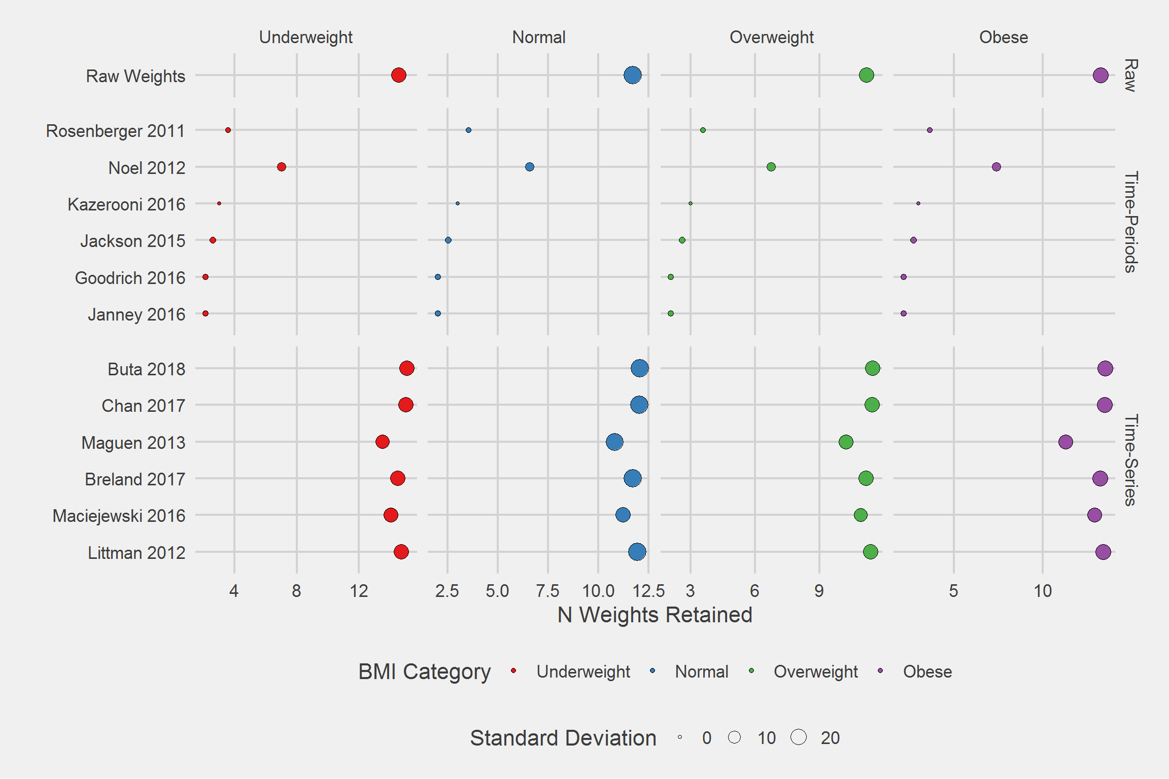
N <- 100
weight_samps <- vector("list", N)
key_cols <- c("Algorithm", "BMI_cat")

pb <- txtProgressBar(min = 0, max = N, initial = 0, style = 3)

for (i in 1:N) {
  setTxtProgressBar(pb, i)
  sampU <- sample(
    pts %>% filter(BMI_cat == "Underweight") %>% pull(PatientICN),
    size = 500, 
    replace = TRUE
  )
  sampN <- sample(
    pts %>% filter(BMI_cat == "Normal") %>% pull(PatientICN),
    size = 500, 
    replace = TRUE
  )
  sampO <- sample(
    pts %>% filter(BMI_cat == "Overweight") %>% pull(PatientICN),
    size = 500, 
    replace = TRUE
  )
  sampOb <- sample(
    pts %>% filter(BMI_cat == "Obese") %>% pull(PatientICN),
    size = 500, 
    replace = TRUE
  )
  samp <- c(sampU, sampN, sampO, sampOb)
  weight_samps[[i]] <- DF %>% filter(PatientICN %in% samp)
  setDT(weight_samps[[i]])
  setkeyv(weight_samps[[i]], key_cols)
  weight_samps[[i]] <- 
    weight_samps[[i]][, 
                      list(mean = mean(Weight), SD = sd(Weight)), 
                      by = key_cols
                      ]
}

Visualization

Distribution of the mean

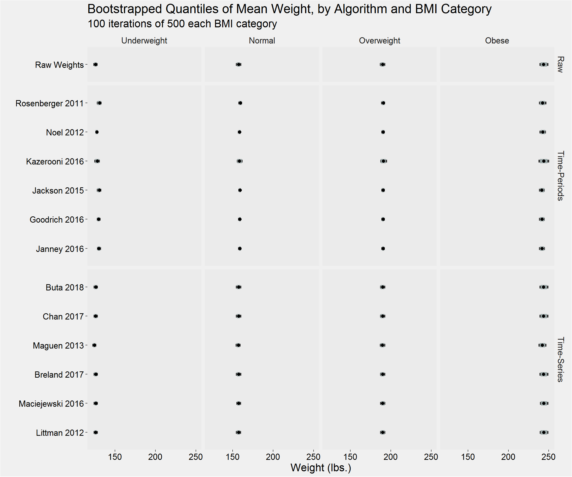
Mean weight does not change much

Distribution of the sample standard deviation,

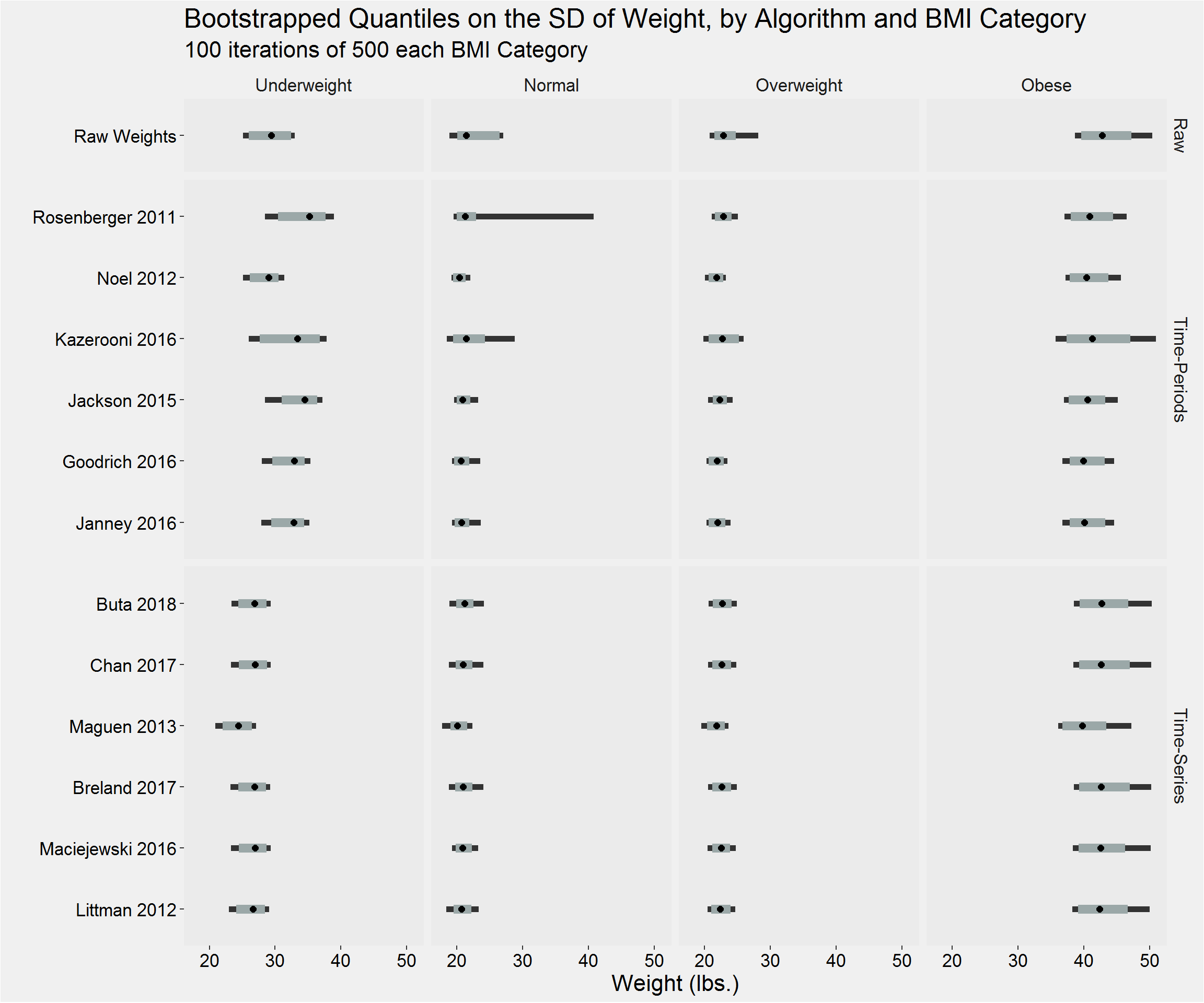
Weight Change Comparison

Add BMI category

DF <- DF %>%
  filter(Cohort == "PCP 2016") %>%
  left_join(
    bmi_cohort %>%
      distinct(PatientICN, BMI_cat),
    by = "PatientICN"
  ) %>%
  na.omit()

Individual Level

Let’s look at the proportions of weight loss \(\geq5\)% from baseline, by algorithm:

DF %>%
  count(Algorithm, BMI_cat, gt5perc_weightloss) %>%
  group_by(Algorithm, BMI_cat) %>%
  mutate(prop = prop.table(n)) %>%
  filter(gt5perc_weightloss == 1) %>%
  select(-gt5perc_weightloss) %>%
  tableStyle()

Algorithm	BMI_cat	n	prop
Raw Weights	Underweight	72	0.20
Raw Weights	Normal	1223	0.15
Raw Weights	Overweight	2595	0.13
Raw Weights	Obese	3378	0.14
Janney 2016	Underweight	69	0.20
Janney 2016	Normal	1176	0.14
Janney 2016	Overweight	2502	0.13
Janney 2016	Obese	3237	0.14
Littman 2012	Underweight	70	0.20
Littman 2012	Normal	1194	0.14
Littman 2012	Overweight	2518	0.12
Littman 2012	Obese	3223	0.13
Maciejewski 2016	Underweight	71	0.21
Maciejewski 2016	Normal	1197	0.15
Maciejewski 2016	Overweight	2556	0.13
Maciejewski 2016	Obese	3297	0.14
Breland 2017	Underweight	72	0.20
Breland 2017	Normal	1221	0.14
Breland 2017	Overweight	2584	0.13
Breland 2017	Obese	3360	0.14
Maguen 2013	Underweight	55	0.18
Maguen 2013	Normal	908	0.12
Maguen 2013	Overweight	1736	0.09
Maguen 2013	Obese	1677	0.08
Goodrich 2016	Underweight	70	0.20
Goodrich 2016	Normal	1175	0.14
Goodrich 2016	Overweight	2497	0.13
Goodrich 2016	Obese	3229	0.14
Chan 2017	Underweight	71	0.20
Chan 2017	Normal	1212	0.14
Chan 2017	Overweight	2572	0.13
Chan 2017	Obese	3336	0.14
Jackson 2015	Underweight	67	0.20
Jackson 2015	Normal	1208	0.14
Jackson 2015	Overweight	2525	0.12
Jackson 2015	Obese	3292	0.14
Buta 2018	Underweight	72	0.20
Buta 2018	Normal	1222	0.15
Buta 2018	Overweight	2588	0.13
Buta 2018	Obese	3365	0.14
Kazerooni 2016	Underweight	58	0.30
Kazerooni 2016	Normal	526	0.16
Kazerooni 2016	Overweight	979	0.13
Kazerooni 2016	Obese	1464	0.14
Noel 2012	Underweight	71	0.21
Noel 2012	Normal	1183	0.15
Noel 2012	Overweight	2460	0.12
Noel 2012	Obese	3218	0.14
Rosenberger 2011	Underweight	53	0.22
Rosenberger 2011	Normal	775	0.15
Rosenberger 2011	Overweight	1732	0.13
Rosenberger 2011	Obese	2335	0.14

Let’s look at the proportions of weight gain \(\geq5\)% from baseline, by algorithm:

DF %>%
  count(Algorithm, BMI_cat, gt5perc_weightgain) %>%
  group_by(Algorithm, BMI_cat) %>%
  mutate(prop = prop.table(n)) %>%
  filter(gt5perc_weightgain == 1) %>%
  select(-gt5perc_weightgain) %>%
  tableStyle()

Algorithm	BMI_cat	n	prop
Raw Weights	Underweight	65	0.18
Raw Weights	Normal	1158	0.14
Raw Weights	Overweight	2173	0.11
Raw Weights	Obese	2662	0.11
Janney 2016	Underweight	59	0.17
Janney 2016	Normal	1120	0.14
Janney 2016	Overweight	2090	0.11
Janney 2016	Obese	2534	0.11
Littman 2012	Underweight	55	0.16
Littman 2012	Normal	1113	0.13
Littman 2012	Overweight	2134	0.10
Littman 2012	Obese	2595	0.11
Maciejewski 2016	Underweight	60	0.18
Maciejewski 2016	Normal	1132	0.14
Maciejewski 2016	Overweight	2131	0.11
Maciejewski 2016	Obese	2583	0.11
Breland 2017	Underweight	60	0.17
Breland 2017	Normal	1153	0.14
Breland 2017	Overweight	2168	0.11
Breland 2017	Obese	2640	0.11
Maguen 2013	Underweight	44	0.14
Maguen 2013	Normal	858	0.11
Maguen 2013	Overweight	1408	0.08
Maguen 2013	Obese	1182	0.06
Goodrich 2016	Underweight	58	0.17
Goodrich 2016	Normal	1119	0.14
Goodrich 2016	Overweight	2086	0.10
Goodrich 2016	Obese	2530	0.11
Chan 2017	Underweight	63	0.18
Chan 2017	Normal	1147	0.14
Chan 2017	Overweight	2154	0.10
Chan 2017	Obese	2624	0.11
Jackson 2015	Underweight	51	0.15
Jackson 2015	Normal	1117	0.13
Jackson 2015	Overweight	2013	0.10
Jackson 2015	Obese	2430	0.10
Buta 2018	Underweight	60	0.17
Buta 2018	Normal	1155	0.14
Buta 2018	Overweight	2172	0.11
Buta 2018	Obese	2649	0.11
Kazerooni 2016	Underweight	24	0.12
Kazerooni 2016	Normal	448	0.14
Kazerooni 2016	Overweight	742	0.10
Kazerooni 2016	Obese	989	0.09
Noel 2012	Underweight	58	0.17
Noel 2012	Normal	1086	0.13
Noel 2012	Overweight	2054	0.10
Noel 2012	Obese	2528	0.11
Rosenberger 2011	Underweight	34	0.14
Rosenberger 2011	Normal	756	0.14
Rosenberger 2011	Overweight	1463	0.11
Rosenberger 2011	Obese	1884	0.12

Average weight change:

DF %>%
  filter(!is.na(diff)) %>%
  select(Algorithm, BMI_cat, diff) %>%
  group_by(Algorithm, BMI_cat) %>%
  summarize(
    mean   = mean(diff),
    SD     = sd(diff),
    min    = min(diff),
    Q1     = fivenum(diff)[2],
    median = median(diff),
    Q3     = fivenum(diff)[4],
    max    = max(diff)
  ) %>%
  tableStyle()

Algorithm	BMI_cat	mean	SD	min	Q1	median	Q3	max
Raw Weights	Underweight	2.24	23.78	-57.00	-4.60	-0.10	3.85	195.80
Raw Weights	Normal	-0.21	10.07	-148.00	-4.80	-0.37	4.00	185.20
Raw Weights	Overweight	-0.54	11.64	-536.00	-5.10	-0.20	4.40	281.97
Raw Weights	Obese	-0.95	15.44	-509.50	-6.80	-0.20	5.80	296.10
Janney 2016	Underweight	0.21	15.44	-57.00	-4.60	-0.25	3.60	195.80
Janney 2016	Normal	-0.20	9.60	-118.60	-4.80	-0.37	4.00	185.20
Janney 2016	Overweight	-0.48	10.68	-291.40	-5.00	-0.20	4.31	281.97
Janney 2016	Obese	-0.97	13.65	-159.20	-6.70	-0.20	5.80	145.50
Littman 2012	Underweight	-0.65	8.78	-34.40	-4.60	-0.30	3.40	31.80
Littman 2012	Normal	-0.31	8.68	-118.60	-4.80	-0.40	4.00	54.70
Littman 2012	Overweight	-0.43	9.25	-67.20	-5.00	-0.20	4.40	70.50
Littman 2012	Obese	-0.75	12.55	-111.80	-6.60	-0.10	5.80	108.00
Maciejewski 2016	Underweight	0.78	17.64	-46.00	-5.00	-0.50	3.70	195.80
Maciejewski 2016	Normal	-0.23	9.09	-55.20	-4.90	-0.40	4.10	70.30
Maciejewski 2016	Overweight	-0.52	9.59	-80.74	-5.20	-0.20	4.50	90.00
Maciejewski 2016	Obese	-0.99	13.07	-117.20	-7.00	-0.20	6.00	99.80
Breland 2017	Underweight	0.16	15.27	-57.00	-4.65	-0.30	3.45	195.80
Breland 2017	Normal	-0.22	9.18	-58.80	-4.80	-0.38	4.00	78.80
Breland 2017	Overweight	-0.49	9.80	-80.86	-5.07	-0.20	4.40	207.20
Breland 2017	Obese	-0.95	13.36	-117.20	-6.70	-0.20	5.80	152.60
Maguen 2013	Underweight	-0.30	7.07	-22.45	-4.35	-0.35	3.10	30.70
Maguen 2013	Normal	-0.24	7.07	-32.00	-4.20	-0.30	3.70	57.00
Maguen 2013	Overweight	-0.38	7.16	-44.50	-4.60	-0.12	4.00	45.00
Maguen 2013	Obese	-0.54	8.59	-73.20	-5.40	-0.10	4.70	98.40
Goodrich 2016	Underweight	-0.37	11.25	-57.00	-4.65	-0.30	3.45	79.00
Goodrich 2016	Normal	-0.21	9.28	-95.10	-4.80	-0.37	4.00	78.80
Goodrich 2016	Overweight	-0.48	9.82	-82.30	-5.00	-0.20	4.30	205.20
Goodrich 2016	Obese	-0.95	13.43	-117.20	-6.70	-0.20	5.80	145.50
Chan 2017	Underweight	1.62	20.83	-46.00	-4.60	-0.15	3.70	195.80
Chan 2017	Normal	-0.19	9.26	-58.80	-4.80	-0.37	4.00	98.12
Chan 2017	Overweight	-0.49	10.16	-245.37	-5.00	-0.20	4.31	278.27
Chan 2017	Obese	-0.96	13.88	-509.50	-6.70	-0.20	5.80	182.15
Jackson 2015	Underweight	-0.13	15.40	-55.75	-5.00	-1.00	3.25	195.80
Jackson 2015	Normal	-0.22	9.42	-156.50	-4.90	-0.40	4.00	199.97
Jackson 2015	Overweight	-0.56	9.68	-245.59	-5.17	-0.38	4.20	230.39
Jackson 2015	Obese	-1.15	13.07	-126.70	-7.00	-0.40	5.50	122.60
Buta 2018	Underweight	0.17	15.29	-57.00	-4.70	-0.30	3.50	195.80
Buta 2018	Normal	-0.21	9.61	-118.60	-4.80	-0.40	4.00	185.20
Buta 2018	Overweight	-0.48	10.27	-245.37	-5.07	-0.20	4.40	278.27
Buta 2018	Obese	-0.94	13.75	-159.20	-6.70	-0.20	5.80	152.60
Kazerooni 2016	Underweight	-1.29	14.04	-28.70	-7.45	-1.20	3.10	142.37
Kazerooni 2016	Normal	-0.40	9.47	-103.30	-5.20	-0.70	4.20	86.20
Kazerooni 2016	Overweight	-0.79	11.58	-534.00	-5.50	-0.60	4.10	154.30
Kazerooni 2016	Obese	-1.40	14.08	-165.97	-7.20	-0.80	5.00	299.30
Noel 2012	Underweight	1.03	18.70	-57.00	-5.00	-0.55	3.50	195.80
Noel 2012	Normal	-0.27	9.13	-128.05	-4.90	-0.40	4.00	84.85
Noel 2012	Overweight	-0.48	9.75	-245.59	-5.00	-0.20	4.40	142.13
Noel 2012	Obese	-0.92	13.26	-119.60	-6.75	-0.20	5.90	145.00
Rosenberger 2011	Underweight	-0.36	12.58	-57.00	-5.20	-0.80	3.20	102.80
Rosenberger 2011	Normal	-0.22	9.62	-141.00	-5.00	-0.50	4.20	78.20
Rosenberger 2011	Overweight	-0.61	11.61	-538.00	-5.30	-0.31	4.50	154.30
Rosenberger 2011	Obese	-1.02	15.42	-509.50	-7.00	-0.20	6.00	298.70

Average Weight Change for those losing \(\ge 5\)% weight loss:

DF %>%
  filter(!is.na(diff) & gt5perc_weightloss == 1) %>%
  select(Algorithm, BMI_cat, diff) %>%
  group_by(Algorithm, BMI_cat) %>%
  summarize(
    mean   = mean(diff),
    SD     = sd(diff),
    min    = min(diff),
    Q1     = fivenum(diff)[2],
    median = median(diff),
    Q3     = fivenum(diff)[4],
    max    = max(diff)
  ) %>%
  tableStyle()

Algorithm	BMI_cat	mean	SD	min	Q1	median	Q3	max
Raw Weights	Underweight	-13.64	8.86	-57.00	-16.00	-11.05	-7.75	-5.00
Raw Weights	Normal	-14.47	9.26	-148.00	-16.45	-12.10	-9.60	-6.00
Raw Weights	Overweight	-17.43	16.44	-536.00	-19.20	-14.10	-11.30	-7.20
Raw Weights	Obese	-23.85	18.99	-509.50	-27.00	-19.00	-14.80	-9.00
Janney 2016	Underweight	-13.88	8.96	-57.00	-16.00	-11.10	-8.00	-5.55
Janney 2016	Normal	-14.20	7.61	-118.60	-16.30	-12.05	-9.60	-6.00
Janney 2016	Overweight	-16.94	11.31	-291.40	-19.00	-14.00	-11.29	-7.20
Janney 2016	Obese	-23.14	13.69	-159.20	-26.80	-19.00	-14.70	-9.00
Littman 2012	Underweight	-12.52	6.06	-34.40	-15.80	-10.91	-7.50	-5.00
Littman 2012	Normal	-13.77	6.45	-118.60	-16.00	-12.00	-9.60	-6.00
Littman 2012	Overweight	-16.08	7.06	-67.20	-18.60	-14.00	-11.20	-7.20
Littman 2012	Obese	-21.71	10.65	-111.80	-25.30	-18.60	-14.60	-9.00
Maciejewski 2016	Underweight	-13.02	7.23	-46.00	-16.00	-11.00	-7.75	-5.00
Maciejewski 2016	Normal	-13.93	6.22	-55.20	-16.30	-12.00	-9.60	-6.00
Maciejewski 2016	Overweight	-16.53	7.98	-80.74	-19.00	-14.00	-11.25	-7.20
Maciejewski 2016	Obese	-22.60	12.28	-117.20	-26.20	-18.80	-14.60	-9.00
Breland 2017	Underweight	-13.64	8.86	-57.00	-16.00	-11.05	-7.75	-5.00
Breland 2017	Normal	-14.08	6.54	-58.80	-16.40	-12.10	-9.60	-6.00
Breland 2017	Overweight	-16.67	8.27	-80.86	-19.05	-14.10	-11.30	-7.20
Breland 2017	Obese	-22.93	12.74	-117.20	-26.85	-19.00	-14.70	-9.00
Maguen 2013	Underweight	-10.10	3.70	-22.45	-11.65	-9.50	-7.30	-5.00
Maguen 2013	Normal	-11.94	4.00	-32.00	-13.80	-11.00	-9.00	-6.00
Maguen 2013	Overweight	-13.71	4.81	-44.50	-15.20	-12.50	-10.70	-7.20
Maguen 2013	Obese	-17.40	6.89	-73.20	-19.30	-15.40	-13.00	-9.00
Goodrich 2016	Underweight	-13.75	8.96	-57.00	-16.00	-11.05	-7.50	-5.00
Goodrich 2016	Normal	-14.11	6.97	-95.10	-16.30	-12.00	-9.60	-6.00
Goodrich 2016	Overweight	-16.66	8.39	-82.30	-19.00	-14.00	-11.20	-7.20
Goodrich 2016	Obese	-22.95	12.98	-117.20	-26.60	-19.00	-14.70	-9.00
Chan 2017	Underweight	-13.03	7.24	-46.00	-16.00	-11.00	-7.75	-5.00
Chan 2017	Normal	-14.01	6.53	-58.80	-16.25	-12.00	-9.60	-6.00
Chan 2017	Overweight	-16.75	9.70	-245.37	-19.00	-14.00	-11.20	-7.20
Chan 2017	Obese	-23.10	15.63	-509.50	-26.61	-19.00	-14.70	-9.00
Jackson 2015	Underweight	-13.80	8.75	-55.75	-16.10	-11.80	-8.15	-5.00
Jackson 2015	Normal	-13.87	7.78	-156.50	-15.77	-11.95	-9.50	-5.90
Jackson 2015	Overweight	-16.36	8.94	-245.59	-18.77	-13.90	-11.30	-6.73
Jackson 2015	Obese	-22.55	12.82	-126.70	-25.59	-18.60	-14.50	-8.35
Buta 2018	Underweight	-13.64	8.86	-57.00	-16.00	-11.05	-7.75	-5.00
Buta 2018	Normal	-14.25	7.62	-118.60	-16.40	-12.10	-9.60	-6.00
Buta 2018	Overweight	-16.85	9.81	-245.37	-19.10	-14.10	-11.30	-7.20
Buta 2018	Obese	-23.17	13.60	-159.20	-27.00	-19.00	-14.70	-9.00
Kazerooni 2016	Underweight	-12.37	5.70	-28.70	-16.00	-10.85	-8.00	-6.00
Kazerooni 2016	Normal	-13.54	7.65	-103.30	-15.20	-11.12	-9.10	-6.00
Kazerooni 2016	Overweight	-16.73	18.99	-534.00	-18.40	-13.60	-11.10	-7.30
Kazerooni 2016	Obese	-22.79	13.07	-165.97	-26.20	-19.00	-14.74	-8.00
Noel 2012	Underweight	-13.13	8.43	-57.00	-16.00	-11.00	-8.03	-5.00
Noel 2012	Normal	-13.86	7.12	-128.05	-16.00	-12.00	-9.50	-6.00
Noel 2012	Overweight	-16.66	9.39	-245.59	-19.17	-14.00	-11.32	-6.95
Noel 2012	Obese	-22.74	12.80	-119.60	-26.01	-18.80	-14.50	-7.40
Rosenberger 2011	Underweight	-13.20	9.27	-57.00	-14.09	-10.70	-8.00	-5.00
Rosenberger 2011	Normal	-14.31	8.38	-141.00	-16.20	-12.10	-9.69	-6.00
Rosenberger 2011	Overweight	-17.60	16.97	-538.00	-19.83	-14.30	-11.40	-7.50
Rosenberger 2011	Obese	-23.98	18.99	-509.50	-27.20	-19.00	-14.70	-9.00

Average Weight Change for those gaining \(\ge 5\)% weight loss:

DF %>%
  filter(!is.na(diff) & gt5perc_weightgain == 1) %>%
  select(Algorithm, BMI_cat, diff) %>%
  group_by(Algorithm, BMI_cat) %>%
  summarize(
    mean   = mean(diff),
    SD     = sd(diff),
    min    = min(diff),
    Q1     = fivenum(diff)[2],
    median = median(diff),
    Q3     = fivenum(diff)[4],
    max    = max(diff)
  ) %>%
  tableStyle()

Algorithm	BMI_cat	mean	SD	min	Q1	median	Q3	max
Raw Weights	Underweight	28.14	45.27	5.50	8.00	11.30	21.61	195.80
Raw Weights	Normal	15.07	10.89	5.00	9.80	12.05	16.80	185.20
Raw Weights	Overweight	16.54	12.92	7.20	11.00	13.50	18.00	281.97
Raw Weights	Obese	21.49	17.19	8.20	14.00	17.60	23.30	296.10
Janney 2016	Underweight	18.20	26.68	5.50	7.95	11.00	18.10	195.80
Janney 2016	Normal	14.82	9.83	5.00	9.80	12.05	16.65	185.20
Janney 2016	Overweight	16.48	12.67	7.20	11.00	13.50	18.00	281.97
Janney 2016	Obese	20.56	11.49	8.20	14.00	17.50	23.00	145.50
Littman 2012	Underweight	12.32	6.33	5.50	7.90	10.30	14.85	31.80
Littman 2012	Normal	13.85	6.43	5.20	9.70	12.00	16.00	54.70
Littman 2012	Overweight	15.66	7.11	7.20	11.00	13.40	18.00	70.50
Littman 2012	Obese	19.90	9.48	8.20	14.00	17.40	22.90	108.00
Maciejewski 2016	Underweight	20.58	32.48	5.45	7.95	11.00	18.65	195.80
Maciejewski 2016	Normal	14.40	7.63	5.20	9.80	12.00	16.60	70.30
Maciejewski 2016	Overweight	15.77	7.35	7.20	11.00	13.50	18.00	90.00
Maciejewski 2016	Obese	19.70	8.83	8.20	13.90	17.30	22.60	99.80
Breland 2017	Underweight	18.05	26.48	5.50	7.95	11.00	18.10	195.80
Breland 2017	Normal	14.61	8.12	5.00	9.80	12.00	16.60	78.80
Breland 2017	Overweight	16.09	9.12	7.20	11.00	13.50	18.00	207.20
Breland 2017	Obese	20.32	10.59	8.20	14.00	17.50	23.00	152.60
Maguen 2013	Underweight	11.11	5.65	5.50	7.55	9.45	11.75	30.70
Maguen 2013	Normal	12.18	5.24	5.20	9.00	11.00	13.60	57.00
Maguen 2013	Overweight	13.12	4.03	7.20	10.38	12.00	14.65	45.00
Maguen 2013	Obese	15.84	5.15	8.20	12.80	14.80	17.80	98.40
Goodrich 2016	Underweight	15.14	12.70	5.50	7.90	11.00	18.00	79.00
Goodrich 2016	Normal	14.67	8.40	5.00	9.80	12.00	16.60	78.80
Goodrich 2016	Overweight	16.14	9.25	7.20	11.00	13.50	18.00	205.20
Goodrich 2016	Obese	20.42	10.95	8.20	14.00	17.40	23.00	145.50
Chan 2017	Underweight	24.53	39.89	5.50	8.00	11.20	20.25	195.80
Chan 2017	Normal	14.70	8.83	5.00	9.80	12.00	16.60	98.12
Chan 2017	Overweight	16.17	10.83	7.20	11.00	13.50	18.00	278.27
Chan 2017	Obese	20.38	11.50	8.20	14.00	17.40	23.00	182.15
Jackson 2015	Underweight	19.07	28.57	5.80	7.89	10.37	19.17	195.80
Jackson 2015	Normal	14.74	9.59	5.74	9.80	12.28	16.60	199.97
Jackson 2015	Overweight	16.02	9.60	6.50	11.00	13.43	18.00	230.39
Jackson 2015	Obese	20.00	10.39	8.00	13.78	17.00	22.80	122.60
Buta 2018	Underweight	18.05	26.48	5.50	7.95	11.00	18.10	195.80
Buta 2018	Normal	14.84	9.78	5.00	9.80	12.00	16.70	185.20
Buta 2018	Overweight	16.32	11.12	7.20	11.00	13.50	18.00	278.27
Buta 2018	Obese	20.69	12.12	8.20	14.00	17.56	23.08	152.60
Kazerooni 2016	Underweight	18.73	27.46	6.50	7.55	11.45	17.75	142.37
Kazerooni 2016	Normal	14.66	8.71	5.80	9.70	12.00	16.15	86.20
Kazerooni 2016	Overweight	16.21	10.17	7.00	10.90	13.60	18.10	154.30
Kazerooni 2016	Obese	21.14	18.80	9.00	13.50	16.60	22.60	299.30
Noel 2012	Underweight	23.55	34.45	5.45	8.70	11.58	21.70	195.80
Noel 2012	Normal	14.49	8.07	5.65	9.70	12.10	16.60	84.85
Noel 2012	Overweight	15.94	8.35	6.95	11.00	13.50	18.00	142.13
Noel 2012	Obese	20.13	10.75	8.20	13.90	17.20	22.87	145.00
Rosenberger 2011	Underweight	18.29	18.77	5.80	7.90	11.50	21.40	102.80
Rosenberger 2011	Normal	14.78	8.16	5.20	10.00	12.40	16.75	78.20
Rosenberger 2011	Overweight	16.37	9.23	7.20	11.00	13.70	18.40	154.30
Rosenberger 2011	Obese	20.89	15.08	7.91	14.00	17.60	23.20	298.70

Visual summaries

p <- DF %>%
  filter(!is.na(diff)) %>%
  ggplot(aes(x = diff, y = Algorithm, fill = Algorithm)) %>% 
  add(ggridges::geom_density_ridges(
    jittered_points = TRUE,
    point_shape = "|",
    position = ggridges::position_points_jitter(height = 0),
    scale = 3, 
    size = 0.25,
    rel_min_height = 10^-5
  )) %>%
  add(facet_grid(Type ~ BMI_cat, scales = "free_y", space = "free_y")) %>%
  add(scale_fill_viridis_d(option = "A")) %>%
  add(theme(
    legend.position = "none",
    text = element_text(size = 20),
    axis.text = element_text(color = "black"),
    panel.grid = element_blank(),
    strip.background = element_blank()
  )) %>%
  add(labs(
      x = "Weight Change (Lbs.)", 
      y = "",
      title = "Weight Change 1-year Post Baseline"
  ))

p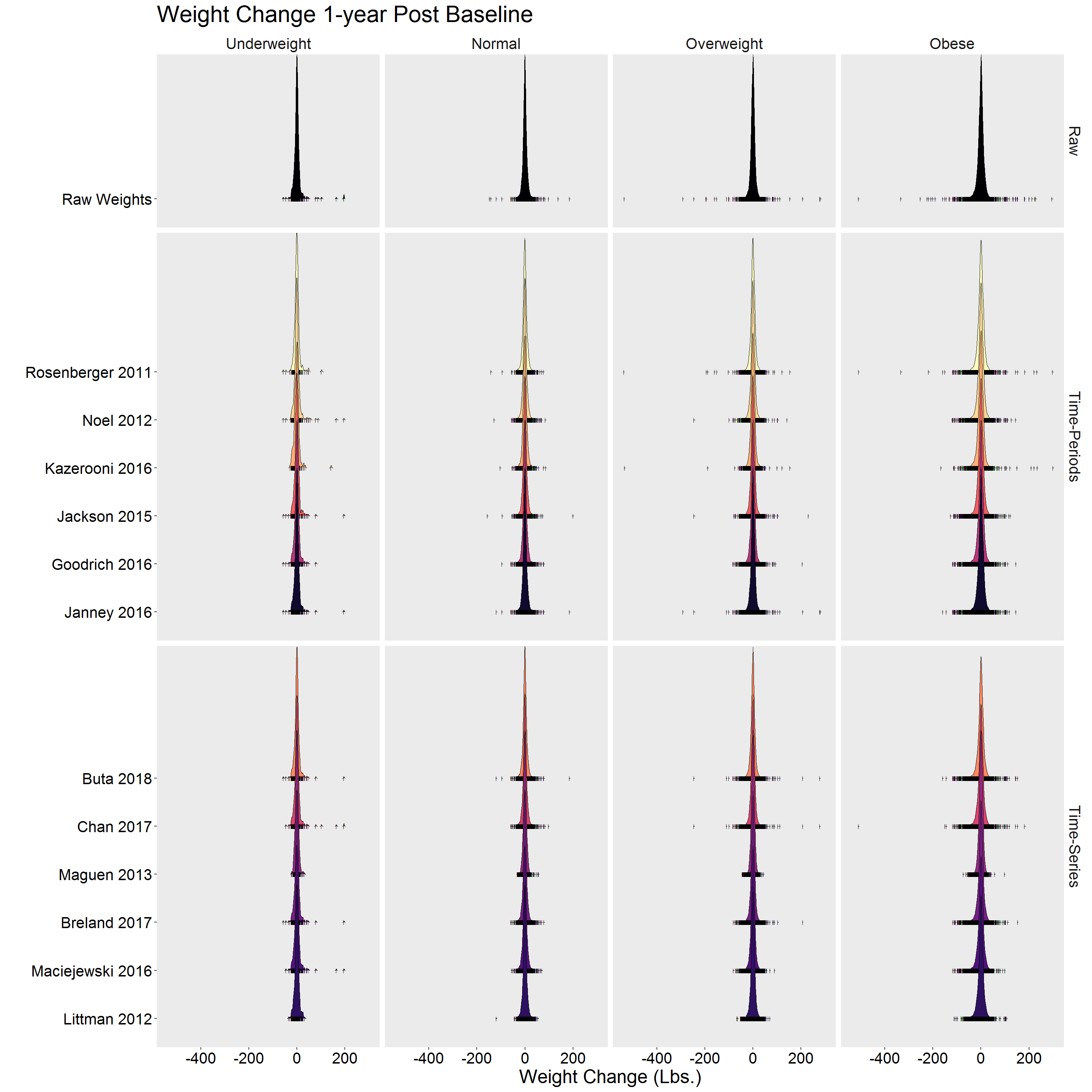

No discernible differences

Alternative view

p <- DF %>%
  filter(!is.na(diff)) %>% 
  group_by(Algorithm) %>% 
  mutate(dens = approxfun(density(diff))(diff)) %>% 
  ggplot(aes(y = Algorithm, x = diff, color = dens)) %>% 
  add(geom_jitter(size = 2)) %>% 
  add(scale_color_viridis_c()) %>% 
  add(facet_grid(Type ~ BMI_cat, scales = "free_y", space = "free_y")) %>%
  add(theme(
    legend.position = "none", 
    text = element_text(size = 20), 
    axis.text = element_text(color = "black"), 
    panel.grid = element_blank(), 
    strip.background = element_blank()
  )) %>%
  add(labs(
      x = "Weight Change (Lbs.)", 
      y = "",
      title = ""
  ))

p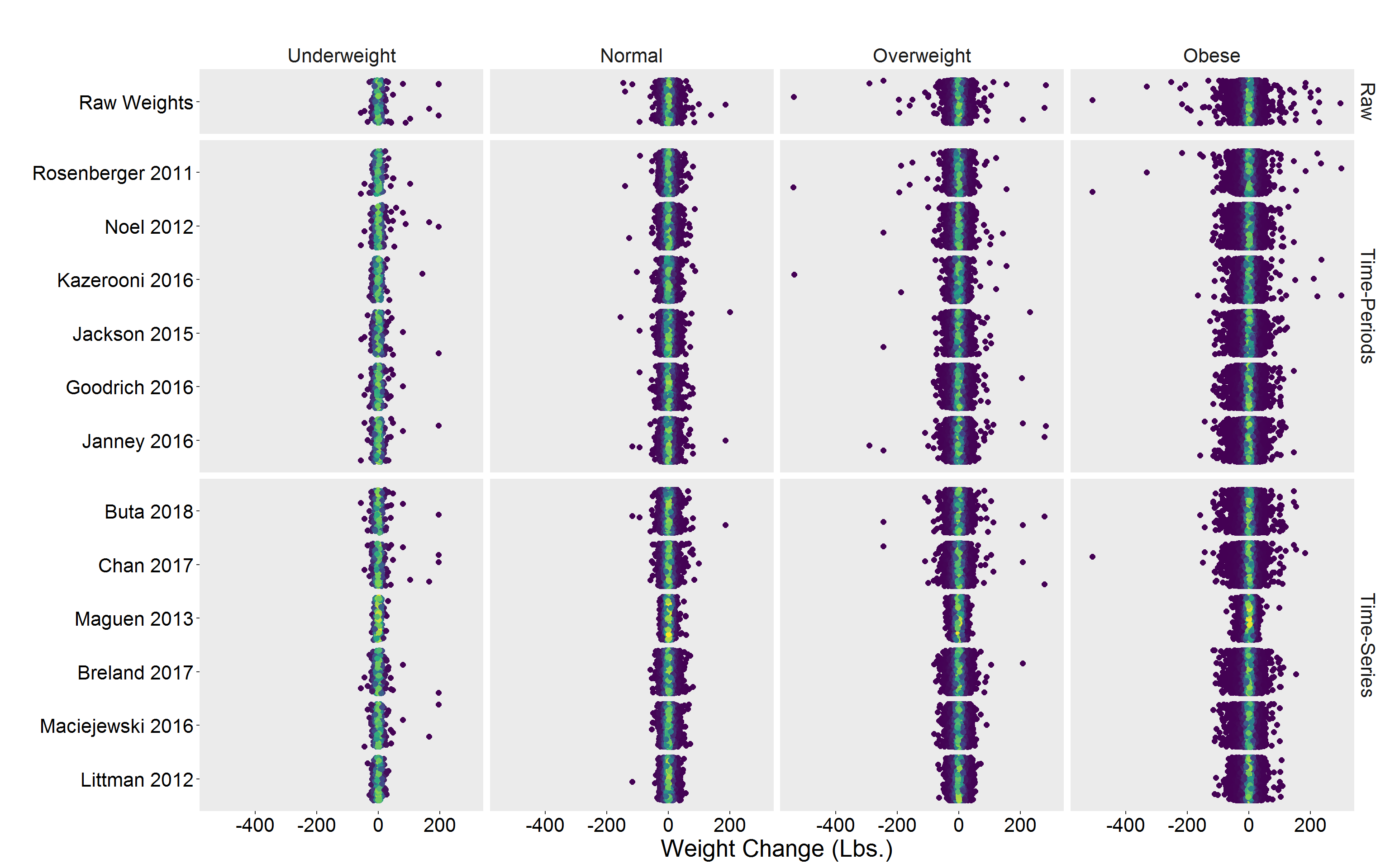

Site/Facility Level Analyses

Sta3n_wtdx_diff <- DF %>%
  select(Algorithm, BMI_cat, Sta3n, diff, diff_perc) %>%
  reshape2::melt(id.vars = c("BMI_cat", "Algorithm", "Sta3n")) %>%
  group_by(BMI_cat, Algorithm, Sta3n, variable) %>%
  na.omit() %>%
  summarize(
    n      = n(),
    mean   = mean(value),
    median = median(value)
  ) %>%
  pivot_wider(
    names_from = variable,
    values_from = c("n", "mean", "median")
  )

Sta3n_wtpct <- DF %>%
  select(BMI_cat, Algorithm, Sta3n, contains("weight")) %>%
  reshape2::melt(id.vars = c("BMI_cat", "Algorithm", "Sta3n")) %>%
  group_by(BMI_cat, Algorithm, Sta3n, variable) %>% 
  summarize(prop = sum(value == 1) / n()) %>% 
  pivot_wider(names_from = variable, values_from = "prop")

Sta3n_wtdx <- Sta3n_wtdx_diff %>%
  left_join(Sta3n_wtpct, by = c("BMI_cat", "Algorithm", "Sta3n")) %>%
  left_join(
    DF %>%
      distinct(Algorithm, Type),
    by = "Algorithm"
  ) %>%
  select(
    Type,
    BMI_cat,
    Sta3n,
    n_diff,
    mean_diff,
    median_diff,
    mean_diff_perc,
    median_diff_perc,
    gt5perc_weightloss,
    gt5perc_weightgain
  ) %>%
  ungroup()

rm(Sta3n_wtdx_diff, Sta3n_wtpct)

COLS <- c("#2E364F", "#2D5D7C", "#F3F0E2", "#EF5939")

p <- Sta3n_wtdx %>%
  ggplot(aes(mean_diff, group = BMI_cat, fill = BMI_cat)) %>%
  add(geom_histogram(bins = 100, alpha = 0.7, color = "black")) %>%
  add(theme_minimal(16)) %>%
  add(theme(legend.position = "none")) %>%
  add(scale_fill_manual(values = COLS)) %>%
  add(labs(
    x = "Weight Change (lbs.)",
    y = "Frequency",
    fill = ""
  ))

q <- Sta3n_wtdx %>%
  filter(!is.infinite(mean_diff_perc)) %>%
  ggplot(aes(mean_diff_perc, group = BMI_cat, fill = BMI_cat)) %>%
  add(geom_histogram(bins = 100, alpha = 0.7, color = "black")) %>%
  add(theme_minimal(16)) %>%
  add(theme(legend.position = c(0.8, 0.8))) %>%
  add(scale_fill_manual(values = COLS)) %>%
  add(labs(
    x = "Weight Change %",
    y = "Frequency",
    fill = ""
  ))

r <- Sta3n_wtdx %>%
  ggplot(aes(gt5perc_weightloss, group = BMI_cat, fill = BMI_cat)) %>%
  add(geom_histogram(bins = 100, alpha = 0.7, color = "black")) %>%
  add(theme_minimal(16)) %>%
  add(theme(legend.position = "none")) %>%
  add(scale_fill_manual(values = COLS)) %>%
  add(labs(
    x = ">= 5% Weight Loss",
    y = "Frequency"
  ))

s <- Sta3n_wtdx %>%
  filter(!is.na(gt5perc_weightgain)) %>%
  ggplot(aes(gt5perc_weightgain, group = BMI_cat, fill = BMI_cat)) %>%
  add(geom_histogram(bins = 100, alpha = 0.7, color = "black")) %>%
  add(theme_minimal(16)) %>%
  add(theme(legend.position = "none")) %>%
  add(scale_fill_manual(values = COLS)) %>%
  add(labs(
    x = ">= 5% Weight Gain",
    y = "Frequency"
  ))

library(patchwork)

p + q + r + s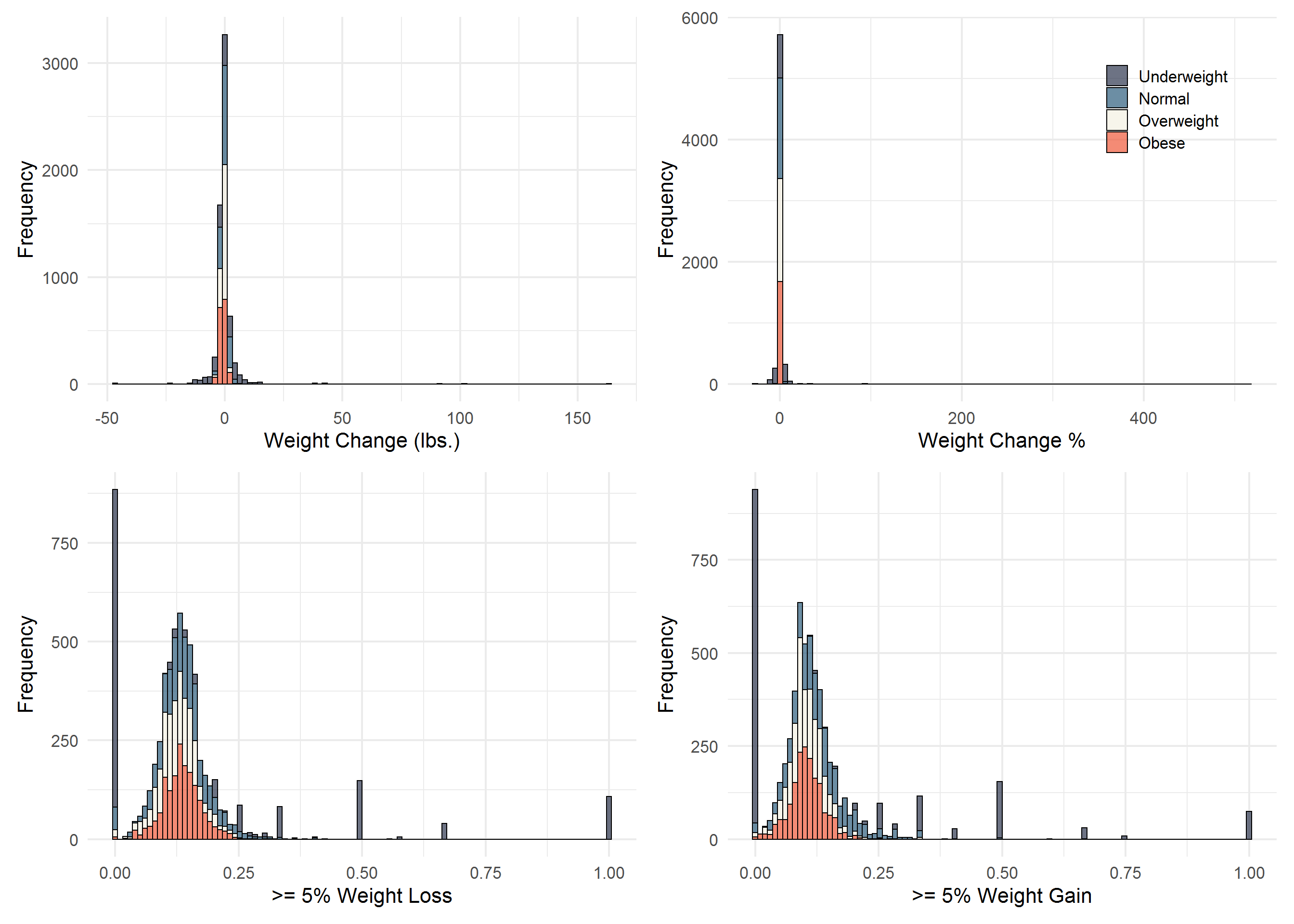

library(gridExtra)

tmp <- Sta3n_wtdx %>%
  select(BMI_cat, Type, Algorithm, Sta3n, gt5perc_weightloss)

raw <- tmp %>% 
  filter(Algorithm == "Raw Weights") %>% 
  group_by(BMI_cat) %>%
  arrange(gt5perc_weightloss) %>%
  mutate(Sta3n_rank = row_number()) %>%
  select(-Type, -Algorithm) %>%
  rename(raw_wtloss = gt5perc_weightloss)

tp <- tmp %>%
  filter(Type == "Time-Periods") %>%
  left_join(raw, by = c("Sta3n", "BMI_cat")) %>%
  mutate(loss_diff = gt5perc_weightloss - raw_wtloss)
  
ts <- tmp %>%
  filter(Type == "Time-Series") %>%
  left_join(raw, by = c("Sta3n", "BMI_cat")) %>%
  mutate(loss_diff = gt5perc_weightloss - raw_wtloss)

p1 <- tp %>%
  ggplot(aes(x = Sta3n_rank, y = raw_wtloss)) %>%
  add(facet_wrap(vars(Type, BMI_cat))) %>%
  add(geom_line(size = 1)) %>%
  add(geom_segment(
    aes(
      x = Sta3n_rank,
      y = raw_wtloss,
      xend = Sta3n_rank,
      yend = gt5perc_weightloss
    ),
    alpha = 0.3
  )) %>%
  add(geom_point(
    aes(
      x = Sta3n_rank, 
      y = gt5perc_weightloss, 
      color = Algorithm
    ),
    size = 2,
    alpha = 0.7
  )) %>%
  add(expand_limits(y = c(0.0, 0.3))) %>%
  add(theme_minimal(16)) %>%
  add(theme(
    legend.position = "bottom",
    panel.grid.major.x = element_blank(),
    panel.grid.minor.x = element_blank()
  )) %>%
  add(guides(color = guide_legend(override.aes = list(size = 5)))) %>%
  add(scale_color_brewer(palette = "Dark2")) %>%
  add(labs(
    x = "Sta3n",
    y = "Proportion Achieving 5% Weight Loss",
    color = ""
  ))

p2 <- p1 %+% ts
p2 <- p2 %>% add(labs(y = ""))
grid.arrange(p1, p2, nrow = 2)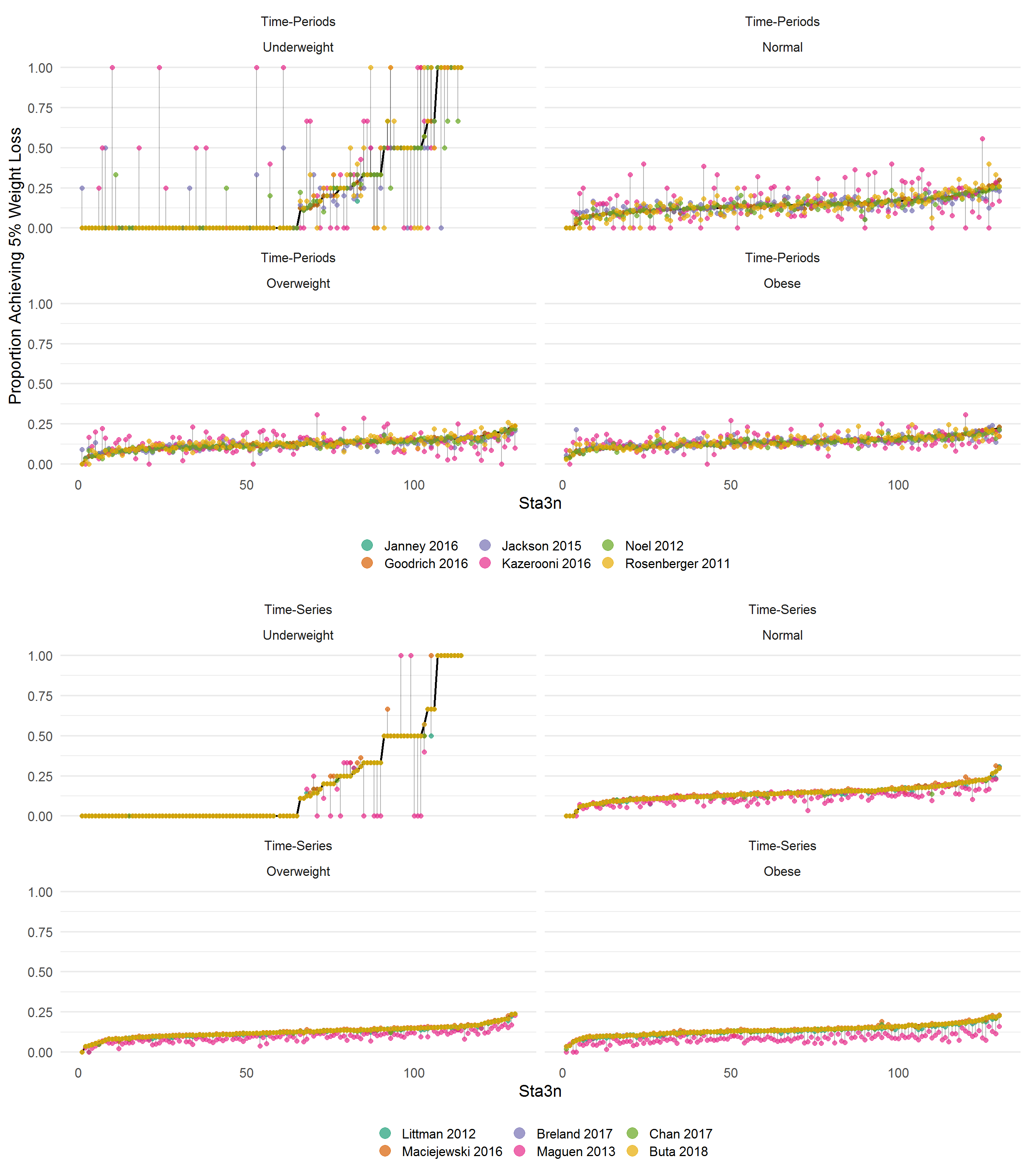

Sites are ordered/ranked along the x-axis using the percent of patients with at least 5% weight loss using the raw data. The left hand side shows the “time-period” algorithms, while the right displays the “time-series” algorithms. Results suggest that generally, time-series algorithms may result in more similar rates by site, save for Maguen 2013. Results are more mixed using the “time-period” algorithms.