Goodrich 2016
Goodrich et al uses a more conservative approach to weight cleaning, where, instead of setting outliers to missing, they completely remove the individual from consideration if they fail to meet the four criteria (see excerpt from published methods).
Excerpt from published methods
…cohort criteria required participants to have a baseline weight documented within 1 month before or after MOVE! enrollment (index date) and at least one follow-up weight at 6 or 12 months after enrollment…Participant records with implausible values for weights (<80 lb or >500 lb) and heights (<48 inches or >84 inches) were excluded, as were those with implausible 6- and 12-month weight changes (>100 lb)
Breakdown of weight measurement removal from cohort:
- Missing enrollment weight (n = 12,589)
- no 6 or 12 month weights (n = 12,870)
- 100+ lb. weight change (n = 3,351)
- Outlier baseline weights (n = 80)
Translation in pseudocode
DEFINE time t_ij for person i IN 1:I, j weights IN 1:J {0mo., 6mo., 12mo.}
FOR i IN 1:I
    weight_i1 := weight @ t_i1 +/- 30 days (baseline)
        IF (weight_i1 == NA)
            EXCLUDE person i
        IF (weight_i1 <= 80 lbs. OR weight_i1 >= 500 lbs.)
            EXCLUDE person i
    FOR j IN 2:J
        weight_ij := weight @ t_ij +/- 60 days
        IF (weight_ij <= 80 lbs. OR weight_ij >= 500 lbs.)
            EXCLUDE person i
    END FOR
    IF (abs(weight_{i, j+1} - weight_{ij}) > 100 lbs.)
        EXCLUDE person i
END FOR
Algorithm in R Code
This code piggybacks off Janney et al 2016, adding only the weight change portion and tweaking the outlier and window functions to suit Goodrich et al.’s specific research needs.
#----------------------- weight change moving forward --------------------------

#' @param DF object of class `data.frame`, containing `id` and `measures`
#' @param id string corresponding to the name of the column of patient identifiers in `DF`
#' @param measures string corresponding to the name of the column of measures in `DF`, e.g., numeric weight data if using to clean weight data
#' @param tmeasures string corresponding to the name of the column of measure dates and/or times in `DF`
#' @param wtchng_thresh numeric scalar used as a cutoff for higher than (or lower than) expected weight changes from one time point j to time point j + 1, by person or group. Default is 100.
lookForwardAndRemove.f <- function(DF,
                                   id,
                                   measures,
                                   tmeasures,
                                   wtchng_thresh = 100) {

  if (!require(data.table)) install.packages("data.table")
  if (!require(dplyr))      install.packages("dplyr")

  # convert to data.table
  DT <- data.table::as.data.table(DF)
  setkeyv(DT, id)

  setorderv(DT, c(id, tmeasures))

  # fast lead with data.table
  DT[,
     "forward" := shift(get(measures),
                        n = 1L,
                        fill = NA,
                        type = "lead"),
     by = id
     ]

  # remove weight changes > wtchng_thresh
  DT$outlier <- abs(DT[[measures]] - DT[["forward"]]) > wtchng_thresh
  DT <- DT %>%
    mutate(
      output = case_when(
        outlier ~ NA_real_,
        is.na(outlier) ~ DT[[measures]],
        TRUE ~ DT[[measures]]
      )
    )

  DT
}

#-------------------- Add weight change to Janney2016.f ---------------------

#' @title Goodrich et al. 2016 Measurment Cleaning Algorithm
#' @param DF object of class data.frame, containing id and weights
#' @param id string corresponding to the name of the column of patient IDs in `DF`
#' @param measures string corresponding to the name of the column of measures in `DF`, e.g., numeric weight data if using to clean weight data
#' @param tmeasures string corresponding to the name of the column of measure dates and/or times in DF
#' @param startPoint string corresponding to the name of the column in `DF` holding the time at which subsequent measurement dates will be assessed, should be the same for each person. Eg., if t = 0 (t[1]) corresponds to an index visit held by the variable 'VisitDate', then startPoint should be set to 'VisitDate'
#' @param t numeric vector of time points to collect measurements, eg. c(0, 182.5, 365) for measure collection at t = 0, t = 180 (6 months from t = 0), and t = 365 (1 year from t = 0). Default is c(0, 182.5, 365) according to Janney et al. 2016
#' @param windows numeric vector of measurement collection windows to use around each time point in t. Eg. Janney et al. 2016 use c(30, 60, 60) for t of c(0, 182.5, 365), implying that the closest measurement t = 0 will be collected 30 days prior to and 30 days post startPoint. Subsequent measurements will be collected 60 days prior to and 60 days post t0+182.5 days, and t0+365 days
#' @param outliers optional. object of type list with numeric inputs corresponding to the upper and lower bound for each time entry in parameter `t`. Default is list(LB = c(80, 80, 80), UB = c(500, 500, 500)) for t = c(0, 182.56, 365), differing between baseline and subsequent measurment collection dates. If not specified then only the subsetting and window functions will be applied.
#' @param wtchng_thresh numeric scalar used as a cutoff for higher than (or lower than) expected weight changes from one time point j to time point j + 1, by person or group. Default is 100.

Goodrich2016.f <- function(DF,
                           id,
                           measures,
                           tmeasures,
                           startPoint,
                           t = c(0, 182, 365),
                           windows = c(30, 60, 60),
                           outliers = list(LB = c(80, 80, 80),
                                           UB = c(500, 500, 500)),
                           wtchng_thresh = 100,
                           excludeSubject = FALSE){

  WindowsAndOutliers.df <-
    Janney2016.f(
      DF,
      id,
      measures,
      tmeasures,
      startPoint,
      t = t,
      windows = windows,
      outliers = outliers
  )

  lookForwardAndRemove.df <-
    lookForwardAndRemove.f(
      DF = WindowsAndOutliers.df,
      id = id,
      measures = "Weight_OR",
      tmeasures = tmeasures,
      wtchng_thresh = wtchng_thresh
    )

  if (excludeSubject) {

    excluded.df <- lookForwardAndRemove.df %>%
      filter(is.na(output)) %>%
      select(id) %>%
      distinct() %>%
      mutate(FlagForRemoval = 1) %>%
      right_join(lookForwardAndRemove.df, by = "PatientICN") %>%
      filter(is.na(FlagForRemoval)) %>%
      select(-FlagForRemoval)

    return(excluded.df)

  } else {
    return(lookForwardAndRemove.df)
  }
}
Algorithm in SAS Code
Example in R
The way I designed this algorithm allows for multiple time points and windows and thus, includes as special cases,
- Hoerster et al. 2014
- Littman et al. 2015
An example Without excluding people due to outliers:
Goodrich2016.df <- Goodrich2016.f(
DF,
id = "PatientICN",
measures = "Weight",
tmeasures = "WeightDateTime",
startPoint = "VisitDateTime"
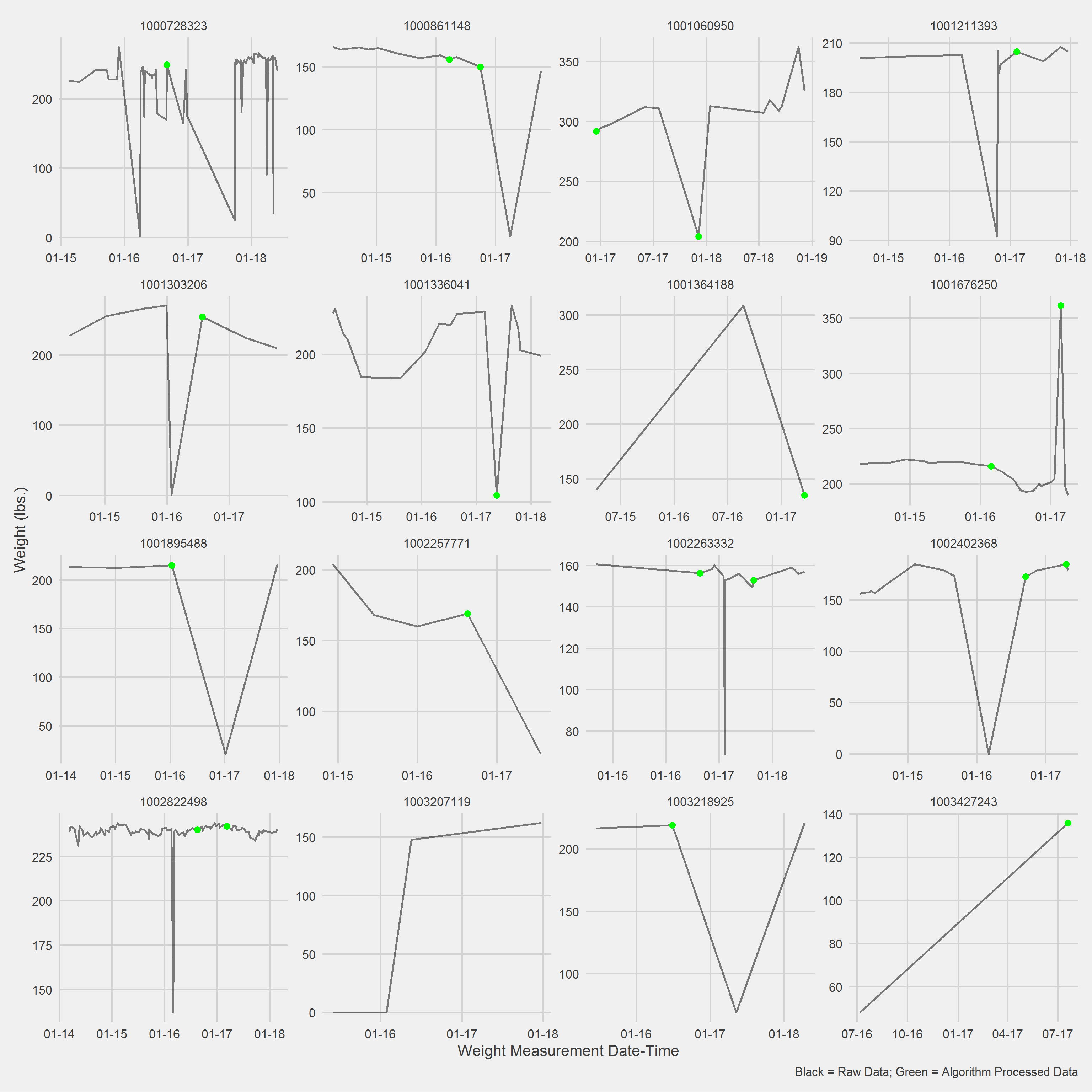
)Displaying a Vignette of 16 selected patients with at least 1 weight observation removed.
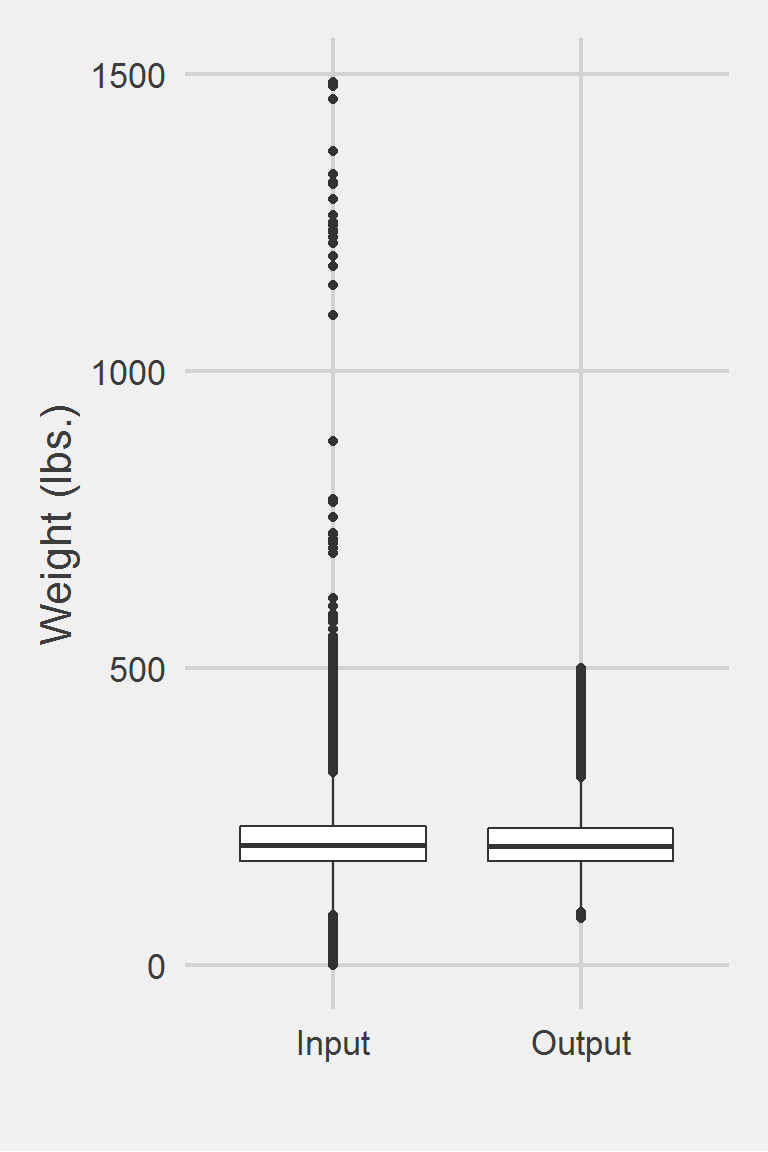
 Descriptive statistics by group
group: Input
   vars       n   mean   sd median trimmed   mad min    max  range skew
X1    1 1175995 207.82 48.6  202.3  204.62 44.18   0 1486.2 1486.2 0.98
   kurtosis   se
X1      5.6 0.04
------------------------------------------------------------
group: Output
   vars      n   mean    sd median trimmed   mad min max range skew kurtosis
X1    1 199786 206.13 45.42    201  203.17 41.51  80 500   420  0.8     1.42
    se
X1 0.1
Left boxplot is raw data from the sample of 2016, PCP visit subjects while the right boxplot describes the output from running Goodrich2016.f()